Chapter8 Chisquare test The mathematical properties of chisquare

Chapter-8 Chi-square test

Ⅰ The mathematical properties of chi-square distribution ð Types of chi-square tests ð Chi-square test ð Chi-square distribution

Types of chi-square tests 1. Tests of goodness-of-fit Observed frequencies of one variable are significantly different from the expected frequencies of the same variable. E. g. occurrences of heads and tails while flipping a coin. 2. Chi-Square tests of independence( or relationship) Two variables are associated or independent of the other. E. g. association between smoking and lung cancer.

Chi-square test ü The chi-square test of independence is probably the most frequently used hypothesis test in the medicine. ü In this chapter, we will use chi-square test to evaluate differences among population when the test variable is nominal, dichotomous, ordinal, or grouped interval.

Independence Defined ü Two variables are independent if, for all cases, the classification of a case into a particular category of one variable (the group variable) has no effect on the probability that the case will fall into any particular category of the second variable (the test variable). ü When two variables are independent, there is no relationship between them. We would expect that the frequency breakdowns of the test variable to be similar for all groups.

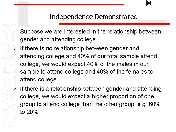
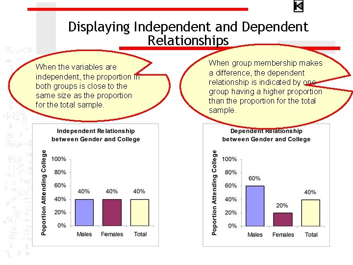
Independence Demonstrated Suppose we are interested in the relationship between gender and attending college. ü If there is no relationship between gender and attending college and 40% of our total sample attend college, we would expect 40% of the males in our sample to attend college and 40% of the females to attend college. ü If there is a relationship between gender and attending college, we would expect a higher proportion of one group to attend college than the other group, e. g. 60% to 20%.

Displaying Independent and Dependent Relationships When the variables are independent, the proportion in both groups is close to the same size as the proportion for the total sample. When group membership makes a difference, the dependent relationship is indicated by one group having a higher proportion than the proportion for the total sample.

Independent and Dependent Variables Ø Ø The two variables in a chi-square test of independence each play a specific role. ü The group variable is also known as the independent variable because it has an influence on the test variable. ü The test variable is also known as the dependent variable because its value is believed to be dependent on the value of the group variable. The chi-square test of independence is a test of the influence or impact that a subject’s value on one variable has on the same subject’s value for a second variable.

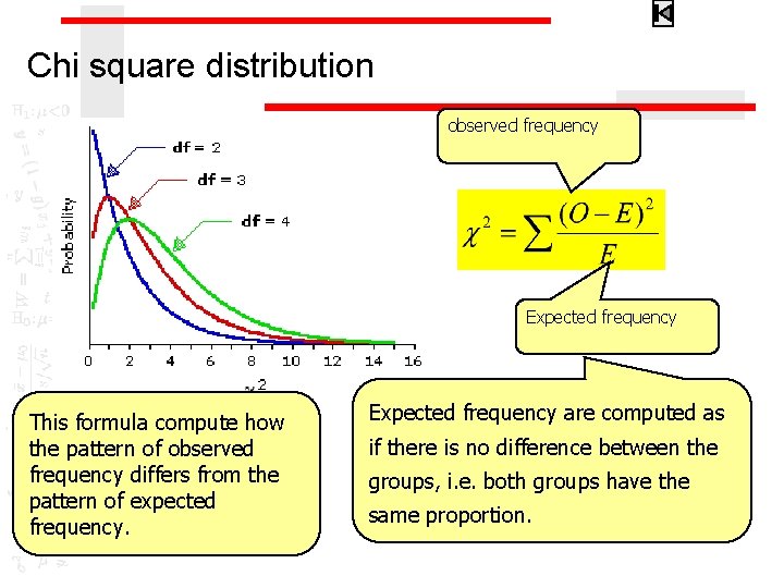
Chi square distribution observed frequency Expected frequency This formula compute how the pattern of observed frequency differs from the pattern of expected frequency. Expected frequency are computed as if there is no difference between the groups, i. e. both groups have the same proportion.

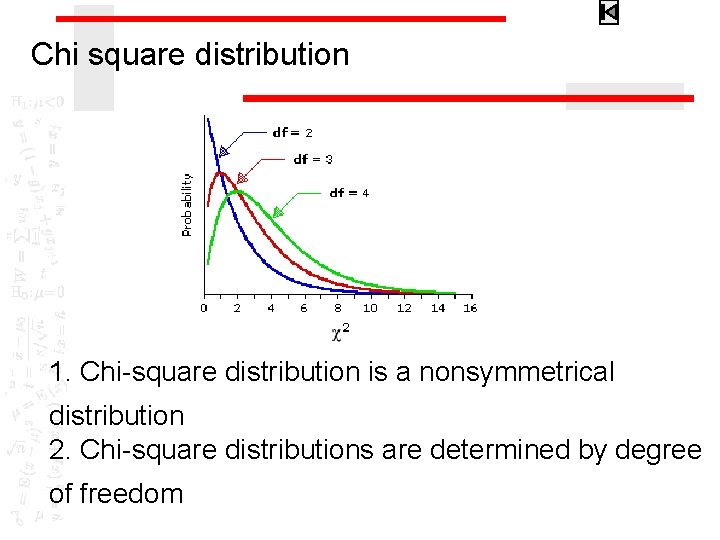
Chi square distribution 1. Chi-square distribution is a nonsymmetrical distribution 2. Chi-square distributions are determined by degree of freedom

Chi square test statistic ü Cannot be negative because all discrepancies are squared. ü Will be zero only in the unusual event that each observed frequency exactly equals the corresponding expected frequency. ü Larger the discrepancy between the expected frequencies and their corresponding observed frequencies, the larger the observed value of chi-square.

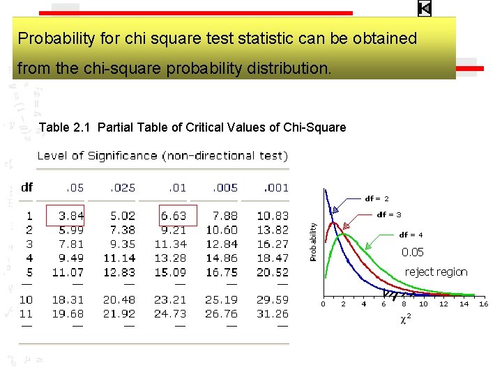
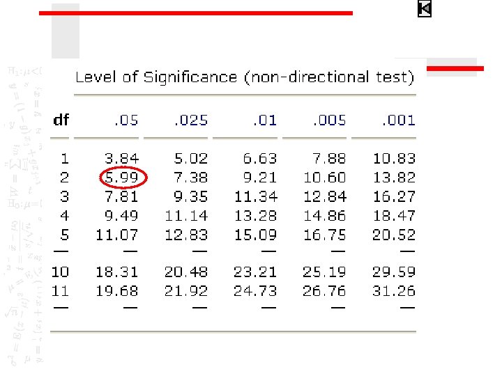
Probability for chi square test statistic can be obtained from the chi-square probability distribution. Table 2. 1 Partial Table of Critical Values of Chi-Square 0. 05 reject region

The decision rule The quantity will be small if the observed and expected frequency are close together and will be large if the differences are large. The computed value of χ2 is compared with the tabulated value of with K-1 degrees of freedom. The decision rule, then is: reject H 0 if χ2 is greater than or equal to the tabulated χ2 for the chosen value of α.

Ⅱ Chi-Square test (tests of goodness-of-fit)

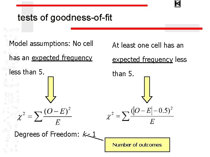
tests of goodness-of-fit Model assumptions: No cell At least one cell has an expected frequency less than 5. Degrees of Freedom: k - 1 Number of outcomes

tests of goodness-of-fit Example 1 As personnel director, you want to test the perception of fairness of three methods of performance evaluation. Of 180 employees, 63 rated Method 1 as fair. 45 rated Method 2 as fair. 72 rated Method 3 as fair. At the 0. 05 level, is there a difference in perceptions?

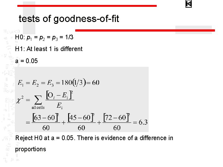
tests of goodness-of-fit H 0: p 1 = p 2 = p 3 = 1/3 H 1: At least 1 is different a = 0. 05 Reject H 0 at a = 0. 05 There is evidence of a difference in proportions

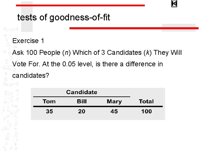
tests of goodness-of-fit Exercise 1 Ask 100 People (n) Which of 3 Candidates (k) They Will Vote For. At the 0. 05 level, is there a difference in candidates?

Ⅲ Chi-Square test (tests of independence or relationship)

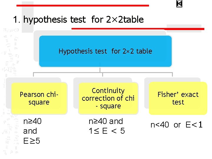
1. hypothesis test for 2× 2 table Hypothesis test for 2× 2 table Pearson chisquare n≥ 40 and E≥ 5 Continuity correction of chi - square Fisher’ exact test n≥ 40 and 1≤ E < 5 n<40 or E<1

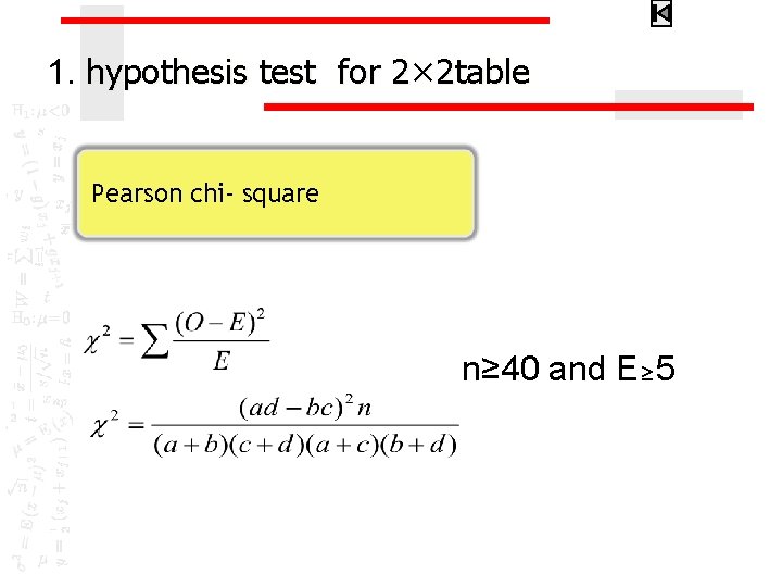
1. hypothesis test for 2× 2 table Pearson chi- square n≥ 40 and E≥ 5

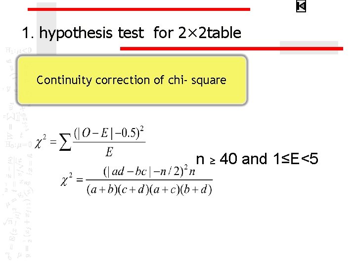
1. hypothesis test for 2× 2 table Continuity correction of chi- square n ≥ 40 and 1≤E<5

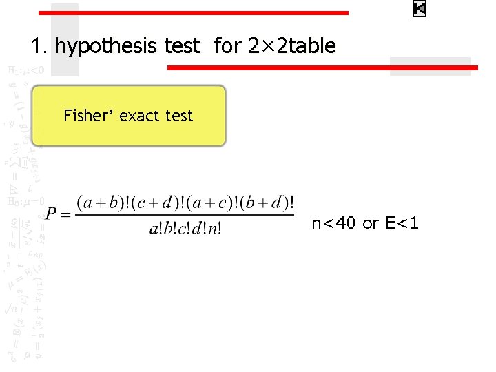
1. hypothesis test for 2× 2 table Fisher’ exact test n<40 or E<1

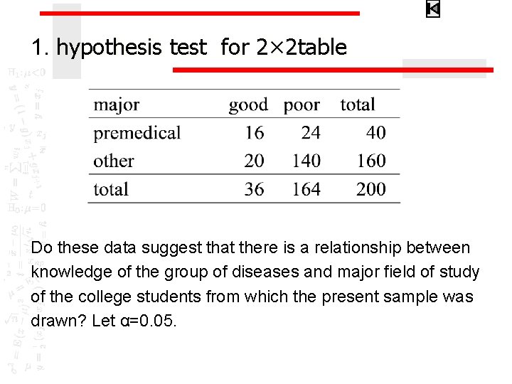
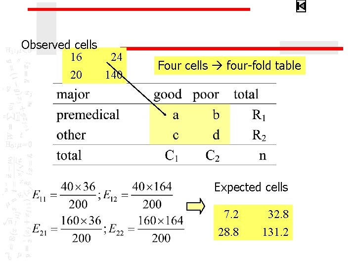
1. hypothesis test for 2× 2 table Example 2 A sample of 200 college students participated in a study designed to evaluate the level of college students’ knowledge of a certain group of common diseases. The following table shows the students classified by major field of study and level of knowledge of the group of diseases:

1. hypothesis test for 2× 2 table Do these data suggest that there is a relationship between knowledge of the group of diseases and major field of study of the college students from which the present sample was drawn? Let α=0. 05.

Observed cells 16 24 20 140 Four cells four-fold table Expected cells 7. 2 28. 8 32. 8 131. 2

1. Chi-Square test for 2× 2 table 16 20 24 140 7. 2 28. 8 H 0: there is no relationship (independent) between knowledge and major field H 1: there is a relationship between knowledge and major field a = 0. 05 32. 8 131. 2

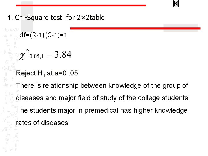
1. Chi-Square test for 2× 2 table df=(R-1)(C-1)=1 Reject H 0 at a=0. 05 There is relationship between knowledge of the group of diseases and major field of study of the college students. The students major in premedical has higher knowledge rates of diseases.

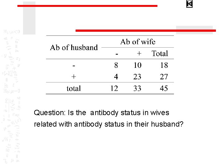
Exercise 2 A study was conducted to determine whether the antibody status in wives is related with antibody status in their husband. 48 couples were examined, the data regarding the incidence of anti- sperm antibodies is as follows:

Question: Is the antibody status in wives related with antibody status in their husband?

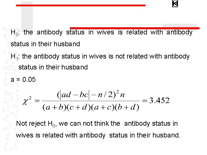
H 0: the antibody status in wives is related with antibody status in their husband H 1: the antibody status in wives is not related with antibody status in their husband a = 0. 05 Not reject H 0, we can not think the antibody status in wives is related with antibody status in their husband.

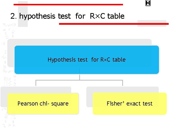
2. hypothesis test for R×C table Hypothesis test for R×C table Pearson chi- square Fisher’ exact test

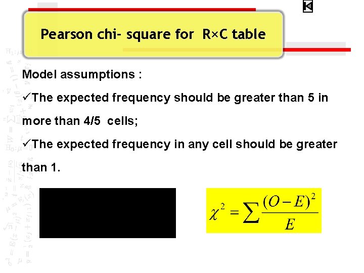
Pearson chi- square for R×C table Model assumptions : üThe expected frequency should be greater than 5 in more than 4/5 cells; üThe expected frequency in any cell should be greater than 1.

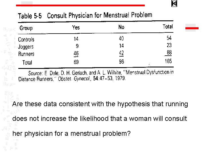
Example 3 To study menstrual dysfunction in distance runners. Somebody did an observational study of three groups of women. The first two groups were volunteers who regularly engaged in some form of running, and the third, a control group, consisted of women who did not run but were otherwise similar to the other two groups. The runners were divided into joggers who jog "slow and easy" 5 to 30 miles per week, and runners who run more than 30 miles per week and combine long, slow distance with speed work. The investigators used a survey to show that the three groups were similar in the amount of physical activity (aside from running), distribution of ages, heights, occupations, and type of birth control methods being used.

Are these data consistent with the hypothesis that running does not increase the likelihood that a woman will consult her physician for a menstrual problem?

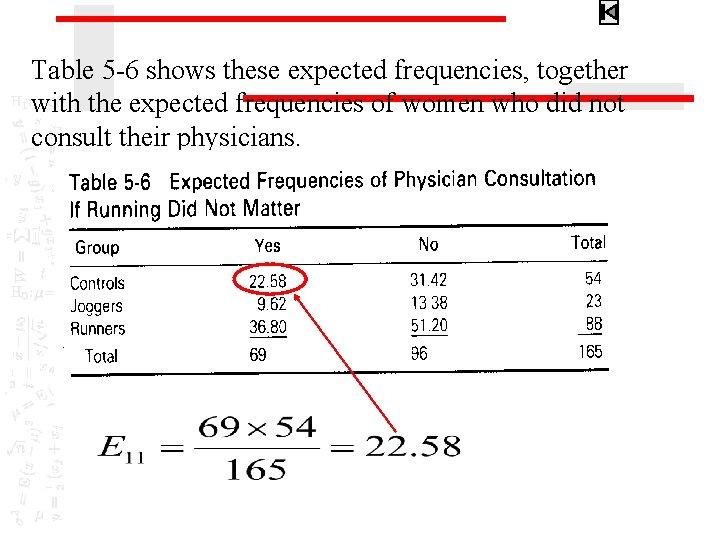
Table 5 -6 shows these expected frequencies, together with the expected frequencies of women who did not consult their physicians.

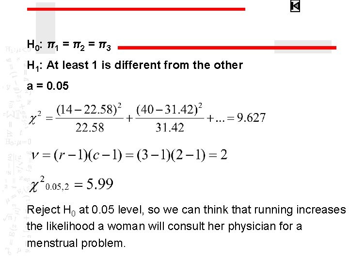
H 0: π 1 = π 2 = π 3 H 1: At least 1 is different from the other a = 0. 05 Reject H 0 at 0. 05 level, so we can think that running increases the likelihood a woman will consult her physician for a menstrual problem.