Principal Component Analysis Mark Stamp PCA 1 Intro

Principal Component Analysis Mark Stamp PCA 1

Intro q Linear algebra based techniques q Can apply directly to binaries o No need for a costly disassembly step q Reveals file structure o But may not be obvious structure q Theory is challenging … q … and training is somewhat complex q But, scoring is fast and very easy PCA 2

Background q The o o following are relevant background Metamorphic techniques Metamorphic malware Metamorphic detection ROC curves q All of these were previously covered, so we’ll skip them q We do cover some basic linear algebra PCA 3

Background q Here, we discuss the following relevant background topics o o o Linear algebra basics Eigenvalues and eigenvectors Basic statistics, covariance matrix Principal Component Analysis (PCA) Singular Value Decomposition (SVD) q And we apply PCA to image recognition and malware detection problems PCA 4

Linear Algebra Basics PCA 5

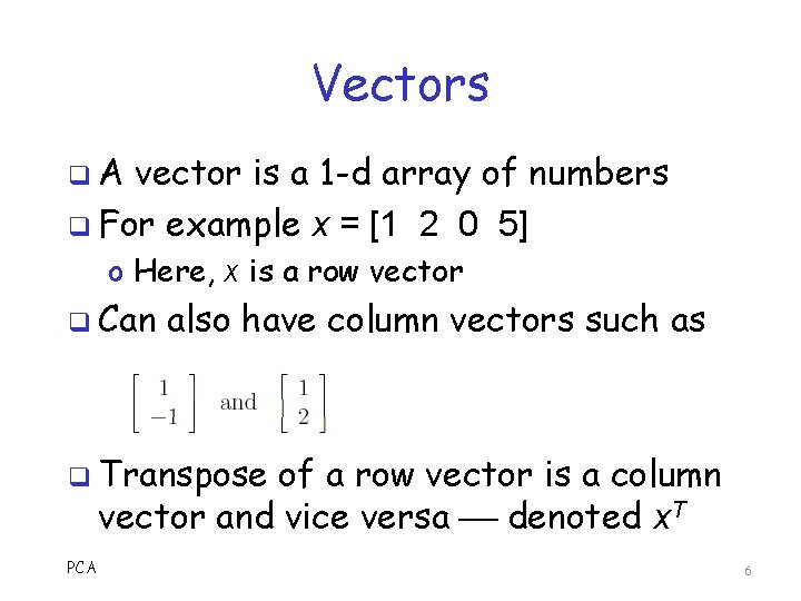
Vectors q. A vector is a 1 -d array of numbers q For example x = [1 2 0 5] o Here, x is a row vector q Can also have column vectors such as q Transpose of a row vector is a column vector and vice versa denoted x. T PCA 6

Dot Product of Vectors q Let X = [x 1 x 2 … xm] and Y = [y 1 y 2 … ym] q Then dot product is defined as o X Y = x 1 y 1 + x 2 y 2 + … + xmym o Note that X Y is a number (scalar) o Also, dot product only defined for vectors of same length q Euclidean distance between X and Y, sqrt((x 1 - y 1)2 + (x 2 - y 2)2 + … + (xm - ym)2) PCA 7

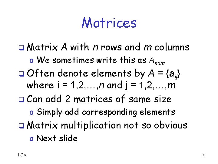
Matrices q Matrix A with n rows and m columns o We sometimes write this as Anxm q Often denote elements by A = {aij} where i = 1, 2, …, n and j = 1, 2, …, m q Can add 2 matrices of same size o Simply add corresponding elements q Matrix multiplication not so obvious o Next slide PCA 8

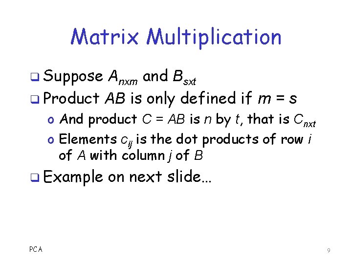
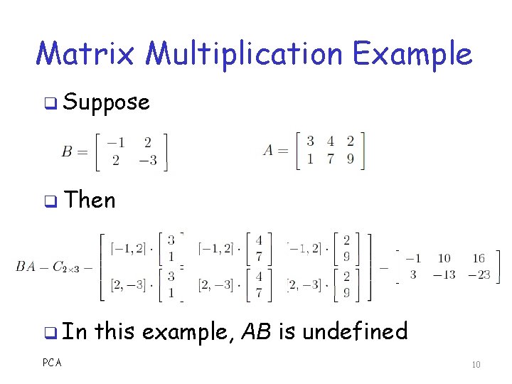
Matrix Multiplication q Suppose Anxm and Bsxt q Product AB is only defined if m = s o And product C = AB is n by t, that is Cnxt o Elements cij is the dot products of row i of A with column j of B q Example PCA on next slide… 9

Matrix Multiplication Example q Suppose q Then q In PCA this example, AB is undefined 10

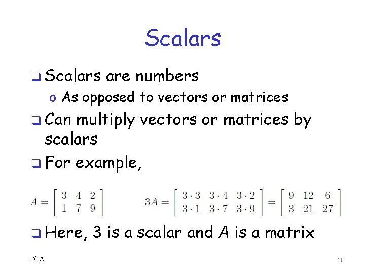
Scalars q Scalars are numbers o As opposed to vectors or matrices q Can multiply vectors or matrices by scalars q For example, q Here, PCA 3 is a scalar and A is a matrix 11

Span q Given a set of vectors, the span consists of all linear combinations q What is a linear combination? o Scalar multiplication and/or sums q Given vectors x and y, their span consists of all vectors ax + by o Here, a and b are scalars PCA 12

Basis q Given a set of vectors… q A basis is a minimal spanning set q That is, no fewer vectors will span q For example, [1 0] and [0 1] form a basis for 2 -d space o Since any [x y] in 2 -d space can be written as [x y] = x [0 1] + y [1 0] q And PCA no one vector is sufficient 13

Eigenvalues and Eigenvectors q In German, “eigen” means “proper” or “characteristic” q Given a matrix A, an eigenvector is a nonzero vector x satisfying Ax = λx o And λ is the corresponding eigenvalue q For eigenvector x, multiplication by A is same as scalar multiplication by λ q So what? PCA 14

Matrix Multiplication Example q Consider the matrix and x = [1 2]T A= q Then Ax = [6 3]T q Not an eigenvector q Can x and Ax align? o Next slide… PCA x Ax 15

Eigenvector Example q Consider the matrix and x = [1 1]T A= q Then Ax = [4 4]T = 4 x q So, x is eigenvector o Of matrix A o With eigenvalue λ = 4 PCA Ax x 16

Eigenvectors q Why are eigenvectors important? o Can “decompose” A by eigenvectors q Matrix A can be written in terms of operations on its eigenvectors o That is, eigenvectors form a basis o And, big eigenvalues most “influential” o Thus, we can reduce dimensionality by ignoring small eigenvalues PCA 17

Statistics 101 PCA 18

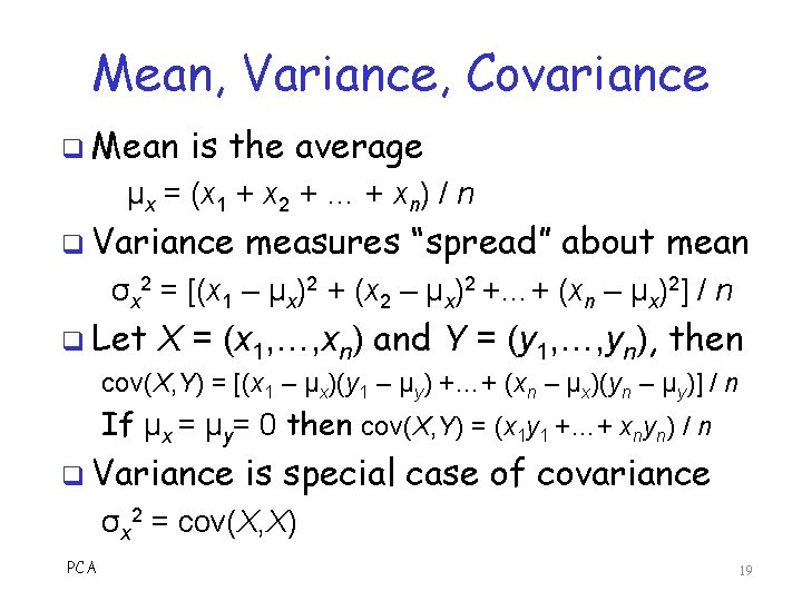
Mean, Variance, Covariance q Mean is the average μx = (x 1 + x 2 + … + xn) / n q Variance measures “spread” about mean σx 2 = [(x 1 – μx)2 + (x 2 – μx)2 +…+ (xn – μx)2] / n q Let X = (x 1, …, xn) and Y = (y 1, …, yn), then cov(X, Y) = [(x 1 – μx)(y 1 – μy) +…+ (xn – μx)(yn – μy)] / n If μx = μy= 0 then cov(X, Y) = (x 1 y 1 +…+ xnyn) / n q Variance is special case of covariance σx 2 = cov(X, X) PCA 19

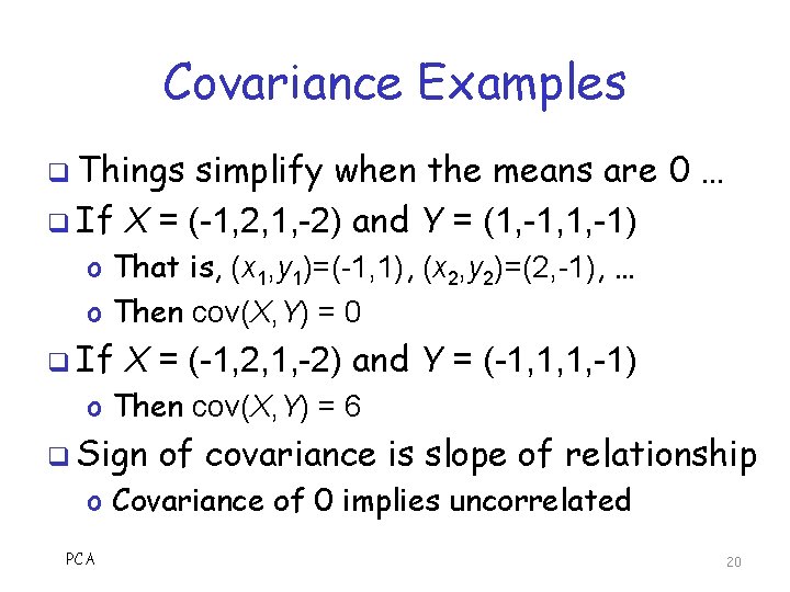
Covariance Examples q Things simplify when the means are 0 … q If X = (-1, 2, 1, -2) and Y = (1, -1, 1, -1) o That is, (x 1, y 1)=(-1, 1), (x 2, y 2)=(2, -1), … o Then cov(X, Y) = 0 q If X = (-1, 2, 1, -2) and Y = (-1, 1, 1, -1) o Then cov(X, Y) = 6 q Sign of covariance is slope of relationship o Covariance of 0 implies uncorrelated PCA 20

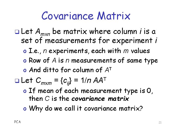
Covariance Matrix q Let Amxn be matrix where column i is a set of measurements for experiment i o I. e. , n experiments, each with m values o Row of A is n measurements of same type o And ditto for column of AT q Let Cmxm = {cij} = 1/n AAT o If mean of each measurement type is 0, then C is the covariance matrix o Why do we call it covariance matrix? PCA 21

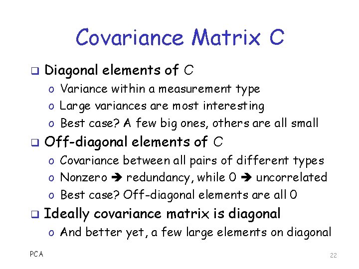
Covariance Matrix C q Diagonal elements of C o Variance within a measurement type o Large variances are most interesting o Best case? A few big ones, others are all small q Off-diagonal elements of C o Covariance between all pairs of different types o Nonzero redundancy, while 0 uncorrelated o Best case? Off-diagonal elements are all 0 q Ideally covariance matrix is diagonal o And better yet, a few large elements on diagonal PCA 22

Principal Component Analysis PCA 23

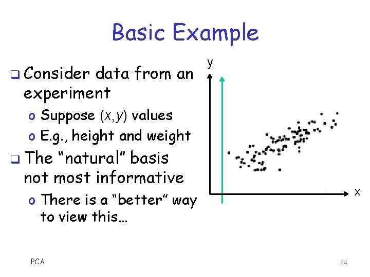
Basic Example q Consider data from an experiment y o Suppose (x, y) values o E. g. , height and weight q The “natural” basis not most informative x o There is a “better” way to view this… PCA 24

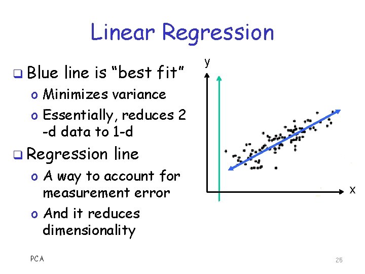
Linear Regression q Blue line is “best fit” y o Minimizes variance o Essentially, reduces 2 -d data to 1 -d q Regression line o A way to account for measurement error o And it reduces dimensionality PCA x 25

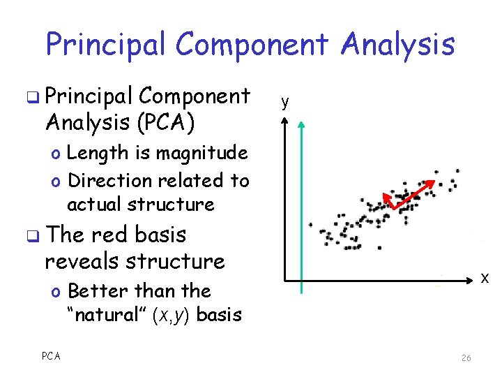
Principal Component Analysis q Principal Component Analysis (PCA) y o Length is magnitude o Direction related to actual structure q The red basis reveals structure x o Better than the “natural” (x, y) basis PCA 26

PCA: The Big Idea q In PCA, align basis with variances o Do this by diagonalizing covariance matrix C Many ways to diagonalize a matrix q PCA uses following for diagonalization 1. Choose direction with max variance 2. Find direction with max variance that is orthogonal to all previously selected 3. Goto 2 (until we run out of dimensions) q Resulting vectors are principal components q PCA 27

PCA Analogy q Suppose we explore a town in Western U. S. using the following algorithm 1. Drive on the longest street 2. When we see another long street, drive on it 3. Continue for a while… q By driving a few streets, we get most of the important information o So, no need to drive all of the streets o Thereby reducing “dimensionality” of problem PCA 28

PCA Assumptions 1. Linearity o Change of basis is linear operation 2. Large variance implies “interesting” o Large variance is “signal”, small is “noise” o May not be valid for some problems 3. Principal components are orthogonal o Makes problem efficiently solvable o Might not be valid in some cases PCA 29

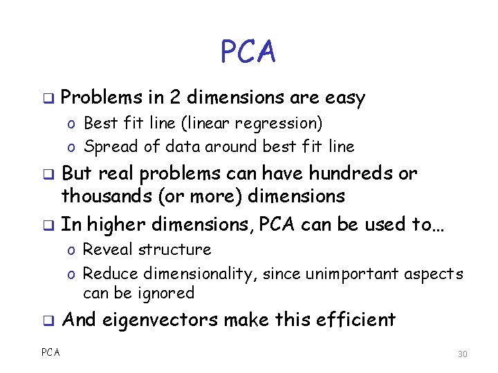
PCA q Problems in 2 dimensions are easy o Best fit line (linear regression) o Spread of data around best fit line But real problems can have hundreds or thousands (or more) dimensions q In higher dimensions, PCA can be used to… q o Reveal structure o Reduce dimensionality, since unimportant aspects can be ignored q PCA And eigenvectors make this efficient 30

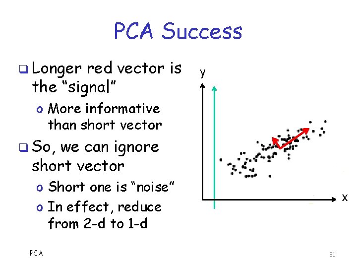
PCA Success q Longer red vector is the “signal” y o More informative than short vector q So, we can ignore short vector o Short one is “noise” o In effect, reduce from 2 -d to 1 -d PCA x 31

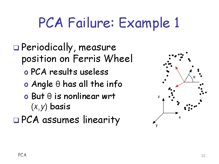
PCA Failure: Example 1 q Periodically, measure position on Ferris Wheel o PCA results useless o Angle θ has all the info o But θ is nonlinear wrt (x, y) basis q PCA assumes linearity 32

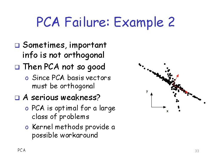
PCA Failure: Example 2 Sometimes, important info is not orthogonal q Then PCA not so good q o Since PCA basis vectors must be orthogonal q A serious weakness? o PCA is optimal for a large class of problems o Kernel methods provide a possible workaround PCA 33

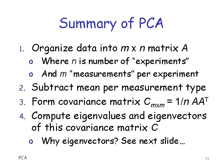
Summary of PCA 1. Organize data into m x n matrix A o Where n is number of “experiments” o And m “measurements” per experiment 2. 3. 4. Subtract mean per measurement type Form covariance matrix Cmxm = 1/n AAT Compute eigenvalues and eigenvectors of this covariance matrix C o Why eigenvectors? See next slide… PCA 34

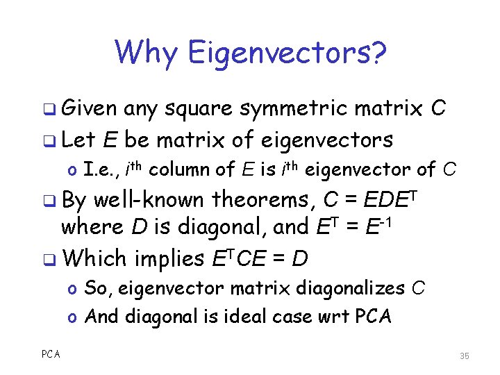
Why Eigenvectors? q Given any square symmetric matrix C q Let E be matrix of eigenvectors o I. e. , ith column of E is ith eigenvector of C q By well-known theorems, C = EDET where D is diagonal, and ET = E-1 q Which implies ETCE = D o So, eigenvector matrix diagonalizes C o And diagonal is ideal case wrt PCA 35

Why Eigenvectors? q We cannot choose the matrix C o Since it comes from the data q So, C won’t be ideal in general o Recall, ideal is diagonal matrix q The best we can do is diagonalize C… o …to reveal “hidden” structure q Lots of ways to diagonalize… o Eigenvectors are an easy way to do so PCA 36

Facial Recognition PCA 37

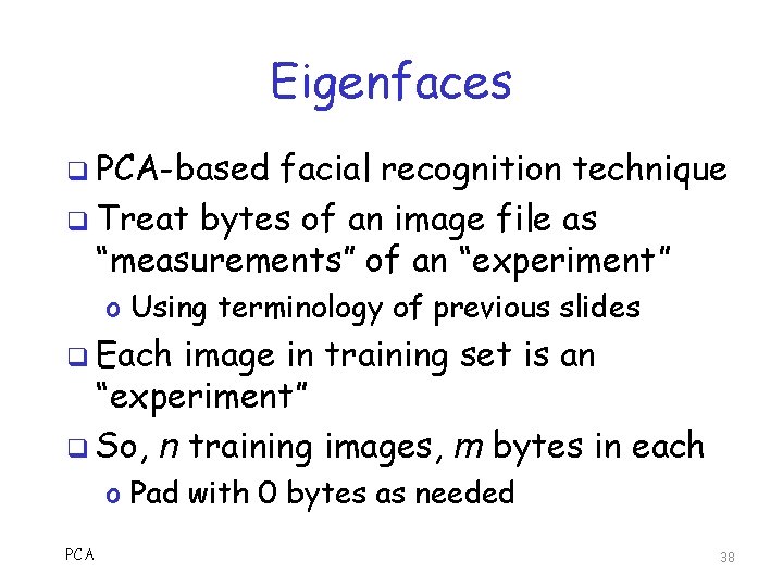
Eigenfaces q PCA-based facial recognition technique q Treat bytes of an image file as “measurements” of an “experiment” o Using terminology of previous slides q Each image in training set is an “experiment” q So, n training images, m bytes in each o Pad with 0 bytes as needed PCA 38

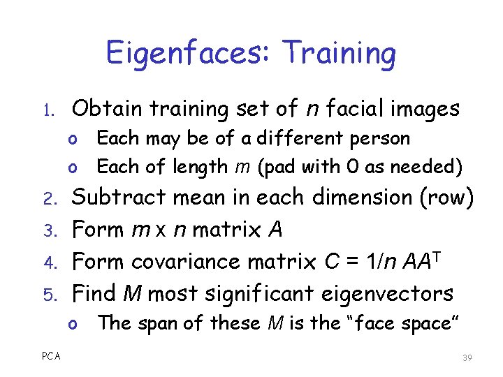
Eigenfaces: Training 1. Obtain training set of n facial images o Each may be of a different person o Each of length m (pad with 0 as needed) 2. 3. 4. 5. Subtract mean in each dimension (row) Form m x n matrix A Form covariance matrix C = 1/n AAT Find M most significant eigenvectors o The span of these M is the “face space” PCA 39

Eigenfaces: Training 6. Compute n vectors of weights o One vector for each training image o Images projected onto face space o Reconstructs images using only the eigenvectors o Resulting vectors are each of length M since M ≤ m eigenvectors used PCA 40

Eigenfaces: Scoring 1. Given an image to score o Measure “closeness” to training set 2. Project image onto face space o Same method as used in training o This was the easy part of training 3. If image is close to anything in the training set, we obtain a low score o And vice versa PCA 41

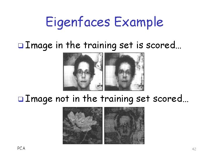
Eigenfaces Example q Image in the training set is scored… q Image not in the training set scored… PCA 42

Eigenfaces: Summary q Training is relatively costly o Must compute eigenvectors q Scoring is fast o Only requires a few dot products q “Face space” contains important info o From the perspective of eigenvectors o But does not necessarily correspond to intuitive features (eyes, nose, etc. ) PCA 43

Malware Detection PCA 44

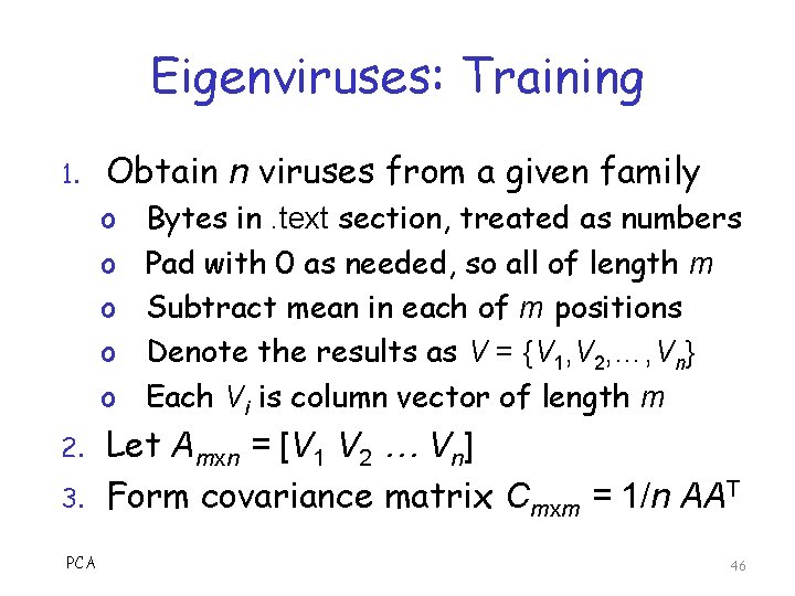
Eigenviruses q PCA-based malware scoring q Treat bytes of an exe file like “measurements” of an “experiment” o We only use bytes in. text section q Each exe in training set is another “experiment” q So, n exe files with m bytes in each o Pad with 0 bytes as needed PCA 45

Eigenviruses: Training 1. Obtain n viruses from a given family o o o 2. 3. PCA Bytes in. text section, treated as numbers Pad with 0 as needed, so all of length m Subtract mean in each of m positions Denote the results as V = {V 1, V 2, …, Vn} Each Vi is column vector of length m Let Amxn = [V 1 V 2 … Vn] Form covariance matrix Cmxm = 1/n AAT 46

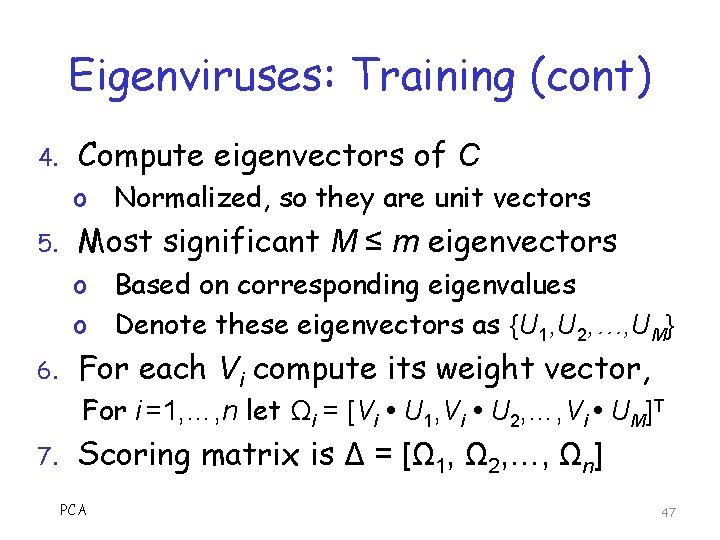
Eigenviruses: Training (cont) 4. Compute eigenvectors of C o Normalized, so they are unit vectors 5. Most significant M ≤ m eigenvectors o Based on corresponding eigenvalues o Denote these eigenvectors as {U 1, U 2, …, UM} 6. For each Vi compute its weight vector, For i =1, …, n let Ωi = [Vi U 1, Vi U 2, …, Vi UM]T 7. Scoring matrix is Δ = [Ω 1, Ω 2, …, Ωn] PCA 47

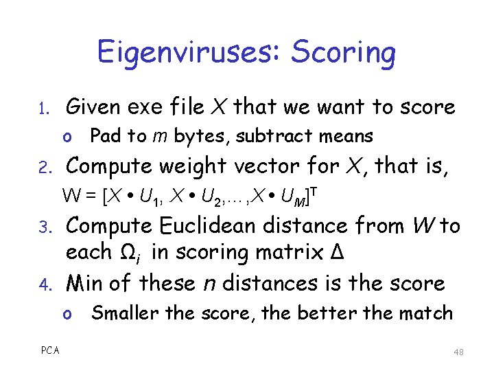
Eigenviruses: Scoring 1. Given exe file X that we want to score o Pad to m bytes, subtract means 2. Compute weight vector for X, that is, W = [X U 1, X U 2, …, X UM]T 3. 4. Compute Euclidean distance from W to each Ωi in scoring matrix Δ Min of these n distances is the score o Smaller the score, the better the match PCA 48

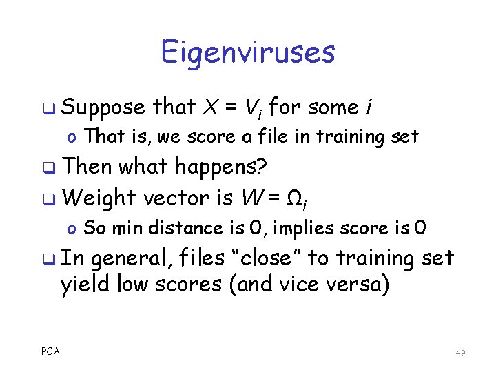
Eigenviruses q Suppose that X = Vi for some i o That is, we score a file in training set q Then what happens? q Weight vector is W = Ωi o So min distance is 0, implies score is 0 q In general, files “close” to training set yield low scores (and vice versa) PCA 49

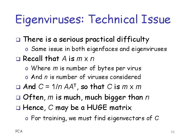
Eigenviruses: Technical Issue q There is a serious practical difficulty o Same issue in both eigenfaces and eigenviruses q Recall that A is m x n o Where m is number of bytes per virus o And n is number of viruses considered And C = 1/n AAT, so that C is m x m q Often, m is much, much bigger than n q Hence, C may be a HUGE matrix q o For training, we must find eigenvectors of C PCA 50

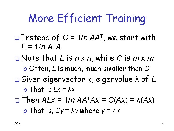
More Efficient Training q Instead of C = 1/n AAT, we start with L = 1/n ATA q Note that L is n x n, while C is m x m o Often, L is much, much smaller than C q Given eigenvector x, eigenvalue λ of L o That is Lx = λx q Then ALx = 1/n AATAx = C(Ax) = λ(Ax) o That is, Cy = λy where y = Ax PCA 51

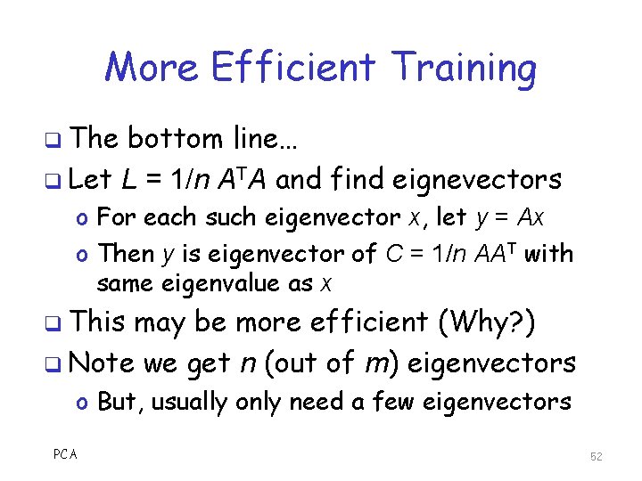
More Efficient Training q The bottom line… q Let L = 1/n ATA and find eignevectors o For each such eigenvector x, let y = Ax o Then y is eigenvector of C = 1/n AAT with same eigenvalue as x q This may be more efficient (Why? ) q Note we get n (out of m) eigenvectors o But, usually only need a few eigenvectors PCA 52

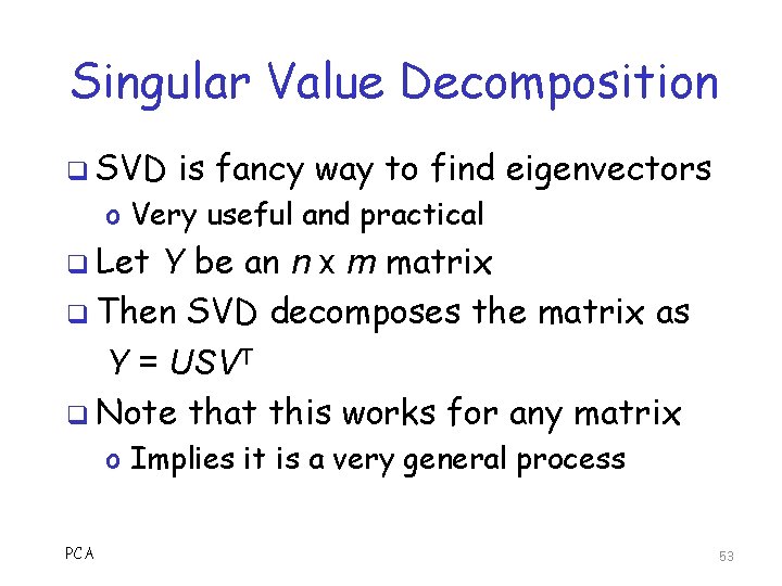
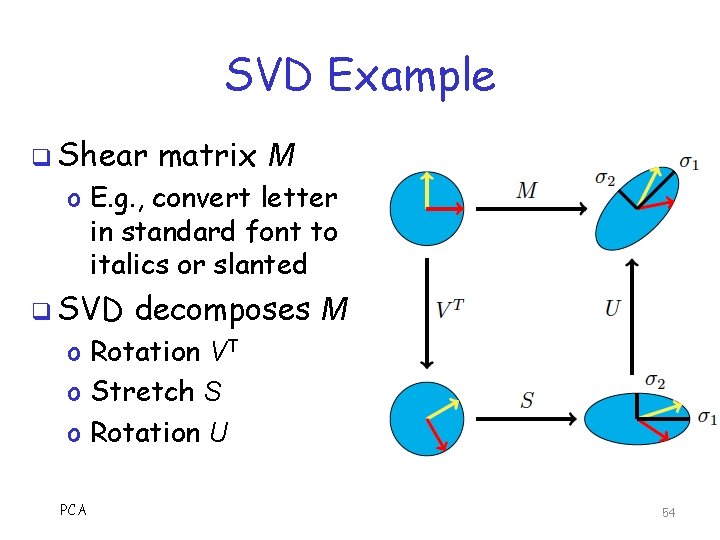
Singular Value Decomposition q SVD is fancy way to find eigenvectors o Very useful and practical q Let Y be an n x m matrix q Then SVD decomposes the matrix as Y = USVT q Note that this works for any matrix o Implies it is a very general process PCA 53

SVD Example q Shear matrix M o E. g. , convert letter in standard font to italics or slanted q SVD decomposes M o Rotation VT o Stretch S o Rotation U PCA 54

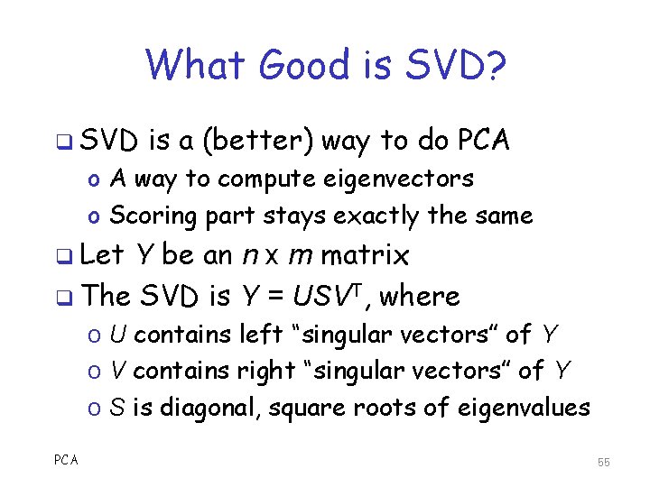
What Good is SVD? q SVD is a (better) way to do PCA o A way to compute eigenvectors o Scoring part stays exactly the same q Let Y be an n x m matrix q The SVD is Y = USVT, where o U contains left “singular vectors” of Y o V contains right “singular vectors” of Y o S is diagonal, square roots of eigenvalues PCA 55

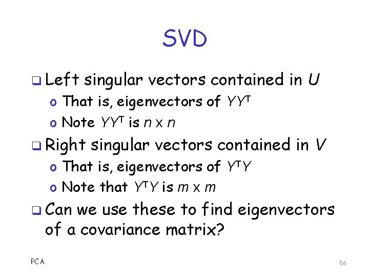
SVD q Left singular vectors contained in U o That is, eigenvectors of YYT o Note YYT is n x n q Right singular vectors contained in V o That is, eigenvectors of YTY o Note that YTY is m x m q Can we use these to find eigenvectors of a covariance matrix? PCA 56

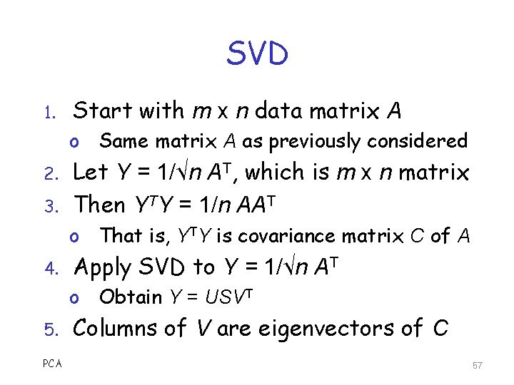
SVD 1. Start with m x n data matrix A o Same matrix A as previously considered 2. 3. Let Y = 1/√n AT, which is m x n matrix Then YTY = 1/n AAT o That is, YTY is covariance matrix C of A 4. Apply SVD to Y = 1/√n AT o Obtain Y = USVT 5. PCA Columns of V are eigenvectors of C 57

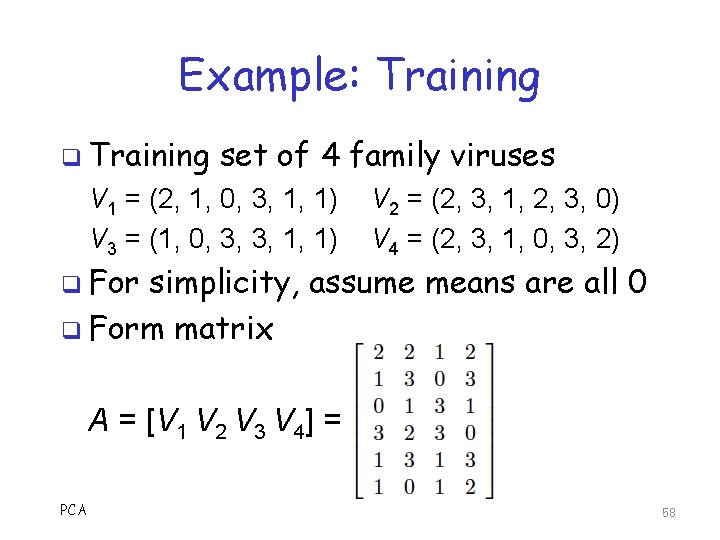
Example: Training q Training set of 4 family viruses V 1 = (2, 1, 0, 3, 1, 1) V 3 = (1, 0, 3, 3, 1, 1) q For V 2 = (2, 3, 1, 2, 3, 0) V 4 = (2, 3, 1, 0, 3, 2) simplicity, assume means are all 0 q Form matrix A = [V 1 V 2 V 3 V 4] = PCA 58

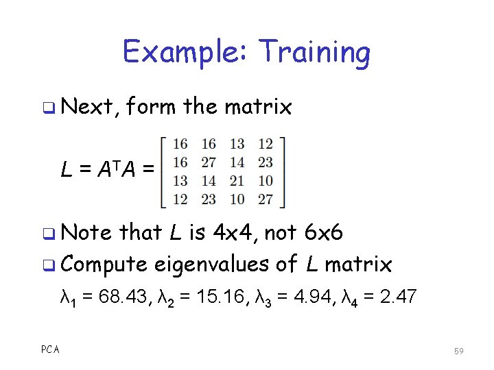
Example: Training q Next, form the matrix L = A TA = q Note that L is 4 x 4, not 6 x 6 q Compute eigenvalues of L matrix λ 1 = 68. 43, λ 2 = 15. 16, λ 3 = 4. 94, λ 4 = 2. 47 PCA 59

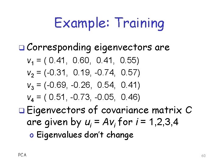
Example: Training q Corresponding eigenvectors are v 1 = ( 0. 41, 0. 60, 0. 41, v 2 = (-0. 31, 0. 19, -0. 74, v 3 = (-0. 69, -0. 26, 0. 54, v 4 = ( 0. 51, -0. 73, -0. 05, 0. 55) 0. 57) 0. 41) 0. 46) q Eigenvectors of covariance matrix C are given by ui = Avi for i = 1, 2, 3, 4 o Eigenvalues don’t change PCA 60

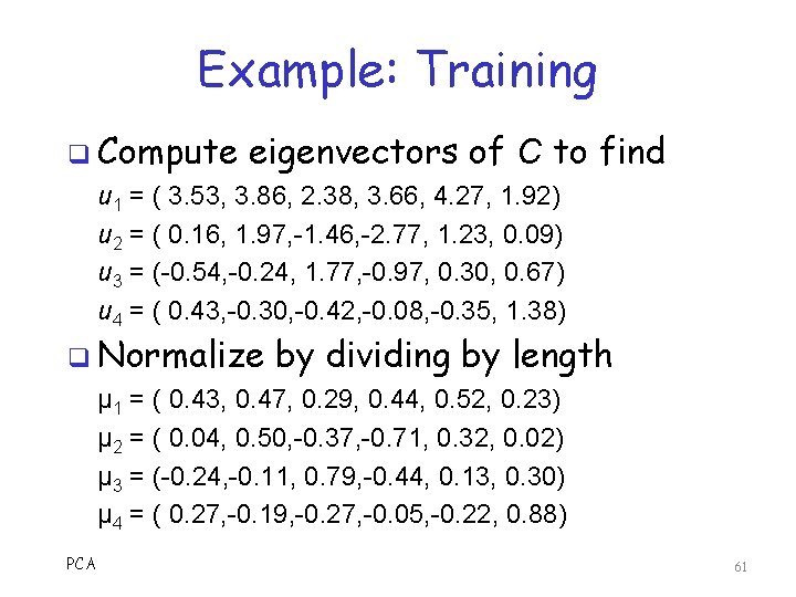
Example: Training q Compute eigenvectors of C to find u 1 = ( 3. 53, 3. 86, 2. 38, 3. 66, 4. 27, 1. 92) u 2 = ( 0. 16, 1. 97, -1. 46, -2. 77, 1. 23, 0. 09) u 3 = (-0. 54, -0. 24, 1. 77, -0. 97, 0. 30, 0. 67) u 4 = ( 0. 43, -0. 30, -0. 42, -0. 08, -0. 35, 1. 38) q Normalize by dividing by length μ 1 = ( 0. 43, 0. 47, 0. 29, 0. 44, 0. 52, 0. 23) μ 2 = ( 0. 04, 0. 50, -0. 37, -0. 71, 0. 32, 0. 02) μ 3 = (-0. 24, -0. 11, 0. 79, -0. 44, 0. 13, 0. 30) μ 4 = ( 0. 27, -0. 19, -0. 27, -0. 05, -0. 22, 0. 88) PCA 61

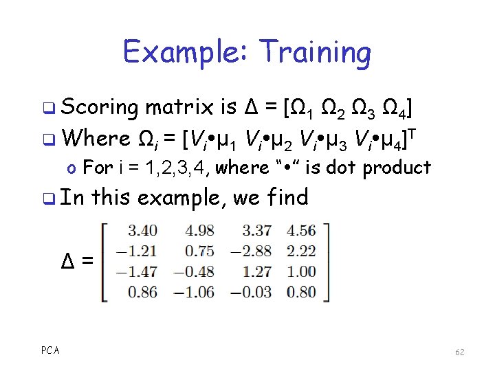
Example: Training q Scoring matrix is Δ = [Ω 1 Ω 2 Ω 3 Ω 4] q Where Ωi = [Vi μ 1 Vi μ 2 Vi μ 3 Vi μ 4]T o For i = 1, 2, 3, 4, where “ ” is dot product q In this example, we find Δ= PCA 62

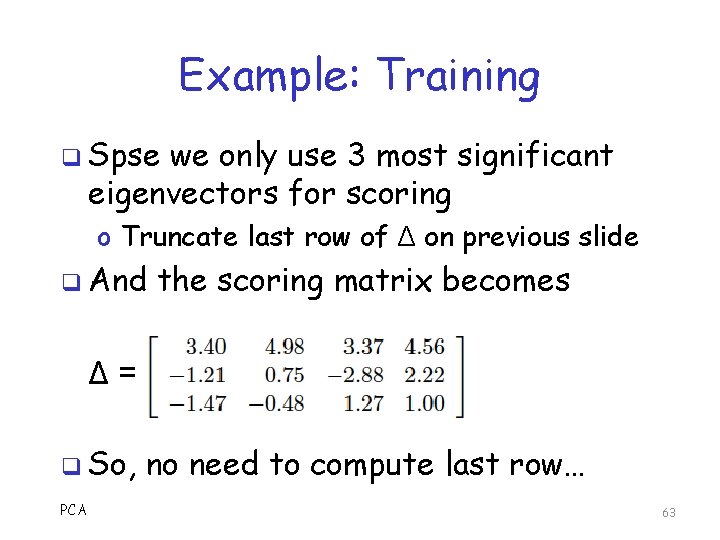
Example: Training q Spse we only use 3 most significant eigenvectors for scoring o Truncate last row of Δ on previous slide q And the scoring matrix becomes Δ= q So, PCA no need to compute last row… 63

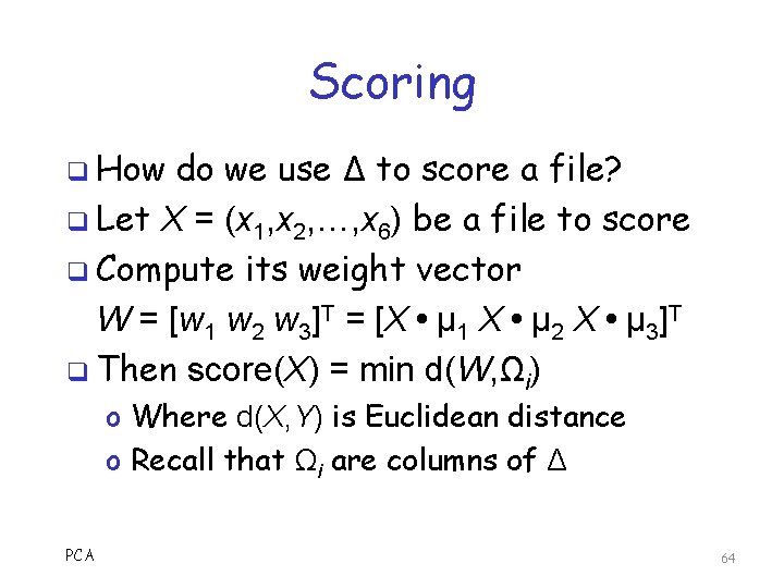
Scoring q How do we use Δ to score a file? q Let X = (x 1, x 2, …, x 6) be a file to score q Compute its weight vector W = [w 1 w 2 w 3]T = [X μ 1 X μ 2 X μ 3]T q Then score(X) = min d(W, Ωi) o Where d(X, Y) is Euclidean distance o Recall that Ωi are columns of Δ PCA 64

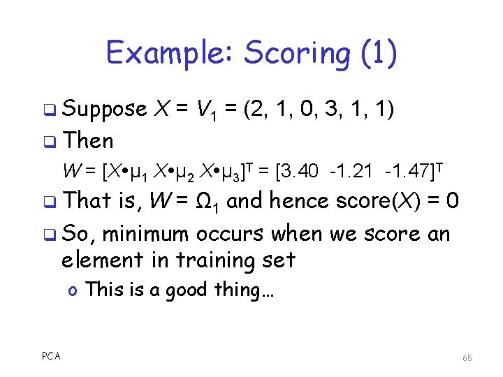
Example: Scoring (1) q Suppose q Then X = V 1 = (2, 1, 0, 3, 1, 1) W = [X μ 1 X μ 2 X μ 3]T = [3. 40 -1. 21 -1. 47]T q That is, W = Ω 1 and hence score(X) = 0 q So, minimum occurs when we score an element in training set o This is a good thing… PCA 65

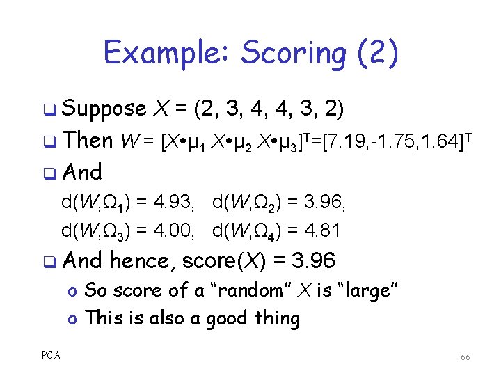
Example: Scoring (2) q Suppose X = (2, 3, 4, 4, 3, 2) q Then W = [X μ 1 X μ 2 X μ 3]T=[7. 19, -1. 75, 1. 64]T q And d(W, Ω 1) = 4. 93, d(W, Ω 2) = 3. 96, d(W, Ω 3) = 4. 00, d(W, Ω 4) = 4. 81 q And hence, score(X) = 3. 96 o So score of a “random” X is “large” o This is also a good thing PCA 66

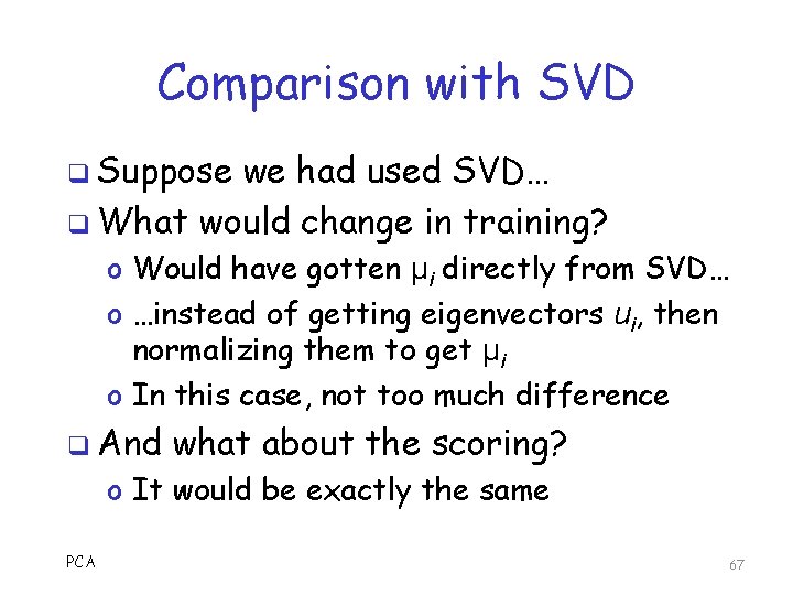
Comparison with SVD q Suppose we had used SVD… q What would change in training? o Would have gotten μi directly from SVD… o …instead of getting eigenvectors ui, then normalizing them to get μi o In this case, not too much difference q And what about the scoring? o It would be exactly the same PCA 67

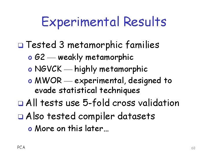
Experimental Results q Tested 3 metamorphic families o G 2 weakly metamorphic o NGVCK highly metamorphic o MWOR experimental, designed to evade statistical techniques q All tests use 5 -fold cross validation q Also tested compiler datasets o More on this later… PCA 68

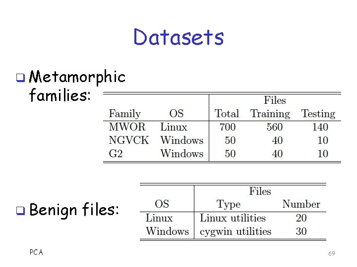
Datasets q Metamorphic families: q Benign PCA files: 69

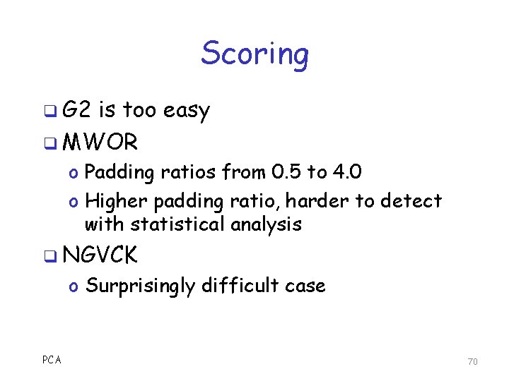
Scoring q G 2 is too easy q MWOR o Padding ratios from 0. 5 to 4. 0 o Higher padding ratio, harder to detect with statistical analysis q NGVCK o Surprisingly difficult case PCA 70

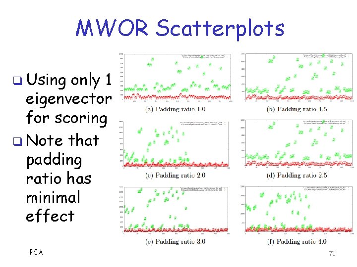
MWOR Scatterplots q Using only 1 eigenvector for scoring q Note that padding ratio has minimal effect PCA 71

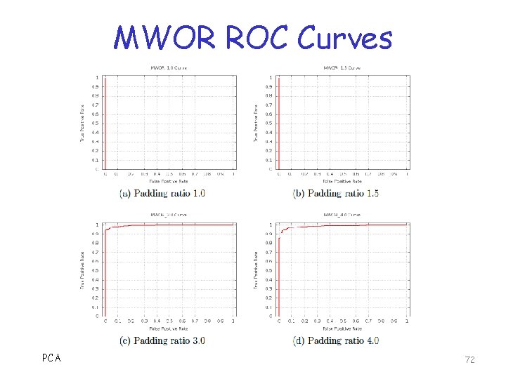
MWOR ROC Curves PCA 72

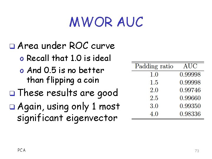
MWOR AUC q Area under ROC curve o Recall that 1. 0 is ideal o And 0. 5 is no better than flipping a coin q These results are good q Again, using only 1 most significant eigenvector PCA 73

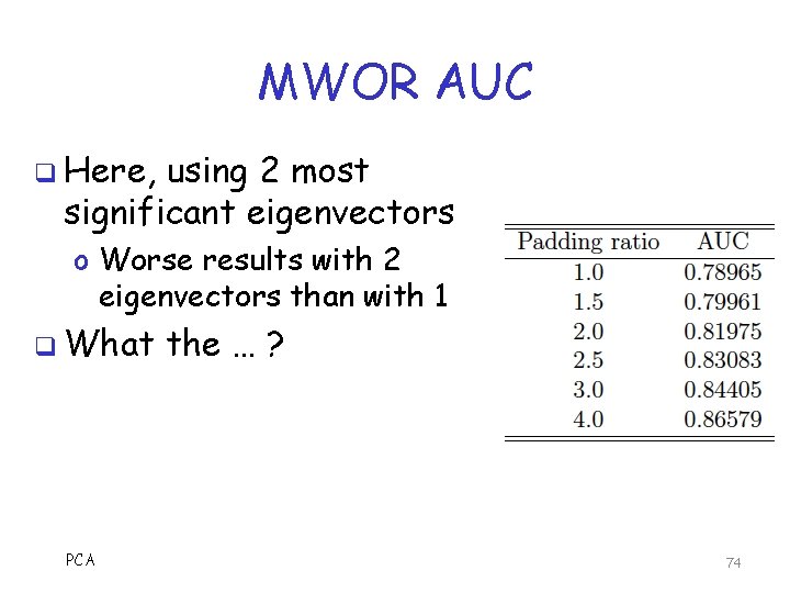
MWOR AUC q Here, using 2 most significant eigenvectors o Worse results with 2 eigenvectors than with 1 q What PCA the … ? 74

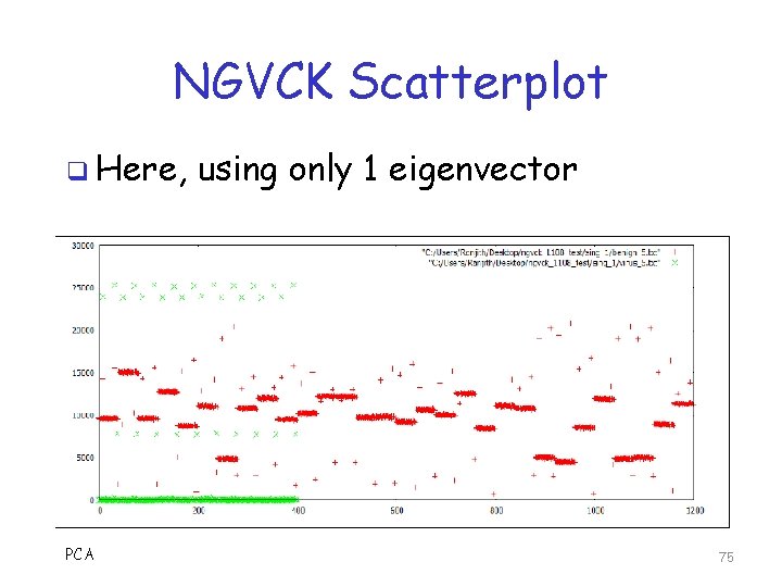
NGVCK Scatterplot q Here, PCA using only 1 eigenvector 75

NGVCK Scoring q Using 1 eigenvector o Get AUC of 0. 91415 q Using 2 eigenvectors o Get AUC of 0. 90282 q Why worse results than MWOR? q What does this say about MWOR and NGVCK viruses? PCA 76

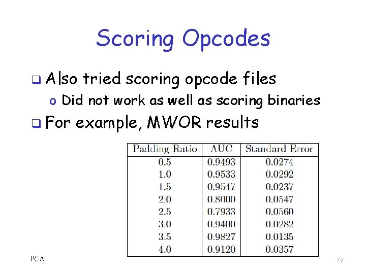
Scoring Opcodes q Also tried scoring opcode files o Did not work as well as scoring binaries q For PCA example, MWOR results 77

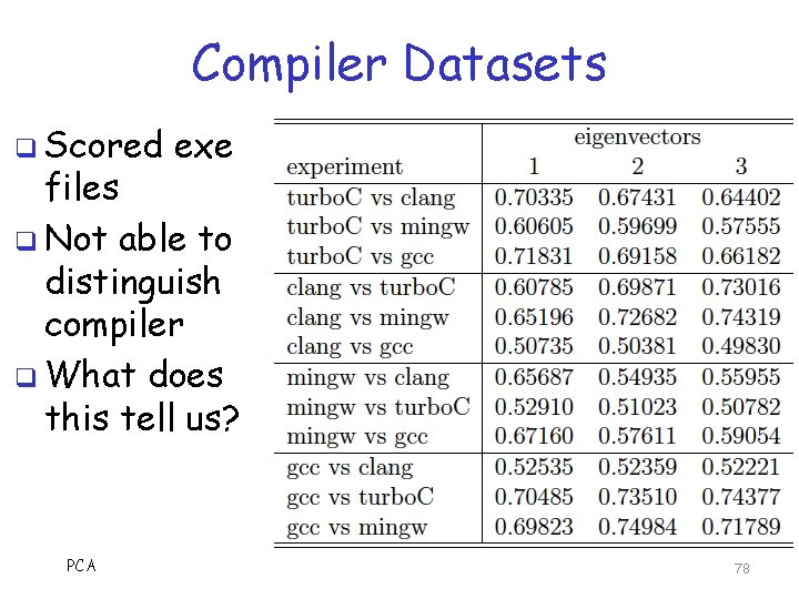
Compiler Datasets q Scored exe files q Not able to distinguish compiler q What does this tell us? PCA 78

Discussion q MWOR results are excellent o Designed to evade statistical detection o Not designed to evade “structural” detection q NGVCK results OK, but not as good o Apparently has some structural variation within the family o But, lots of statistical similarity PCA 79

Discussion q Compiler datasets not distinguishable by eigenvector analysis q Compiler opcodes can be distinguished using statistical techniques (HMMs) o Compilers have statistically “fingerprint” wrt opcodes in asm files o But file structure differs a lot o File structure depends on source code o So this result makes sense PCA 80

Conclusions q Eigenvector techniques very powerful q Theory is fairly complex… q Training is somewhat involved… q But, scoring is simple, fast, efficient q Wrt malware detection o PCA is powerful structure-based score o How might a virus writer defeat PCA? o Hint: Think about compiler results… PCA 81

Future Work q Variations on scoring technique o Other distances, such as Mahalanobis distance, edit distance, … q Better metamorphic generators o Today, none can defeat both statistical and structural scores o How to defeat PCA-based score? q And PCA ? ? ? 82

References: PCA J. Shlens, A tutorial on principal component analysis, 2009 q M. Turk and A. Petland, Eigenfaces for recognition, Journal of Cognitive Neuroscience, 3(1): 71 -86, 1991 q PCA 83

References: Malware Detection q q q PCA M. Saleh, et al, Eigenviruses for metamorphic virus recognition, IET Information Security, 5(4): 191 -198, 2011 S. Deshpande, Y. Park, and M. Stamp, Eigenvalue analysis for metamorphic detection, Journal of Computer Virology and Hacking Techniques, 10(1): 53 -65, 2014 R. K. Jidigam, T. H. Austin, and M. Stamp, Singular value decomposition and metamorphic detection, to appear in Journal of Computer Virology and Hacking Techniques 84