Principle Component Analysis Royi Itzhack Algorithms in computational

Matrix arithmetic, etc. l Product A*B l Transpose A’ l Inverse A^(-1) or inv(A)

The dimension problem l l l Suppose , we want to calculate the probability

The dimension problem l l l Some features are not informative Constant feature –

Algebraic Interpretation – 1 D l Given m points in a n dimensional space,

Algebraic Interpretation – 1 D l l l Given m points in a n

Principal Components l l 25 Wavelength 2 All principal components (PCs) start at the

Covariance Matrix l l l Each i, j is the cov(xi, xj) Each i,

The Algorithm l Step 1: Calculate the Covariance Matrix of the observation matrix. l

PCA – Step 1: Covariance Matrix C Ø - Data Matrix

Linear Algebra Review – Eigenvalue and Eigenvector eigenvector l C - a square n

PCA – Step 3 l Sort eigenvectors by the magnitude of their eigenvalues

PCA – Step 4 l Project the input data onto the principal components. l

PCA: General From k original variables: x 1, x 2, . . . ,

2 nd Principal Component, y 2 1 st Principal Component, y 1

PCA: Another Explanation From k original variables: x 1, x 2, . . .

Example from 2005 b Perform pca for the following data sets X=(0, 0), (1,

Slides: 40

Download presentation

Principle Component Analysis Royi Itzhack Algorithms in computational biology

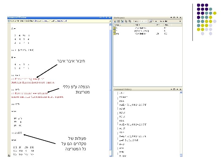
Matrix arithmetic, etc. l Product A*B l Transpose A’ l Inverse A^(-1) or inv(A) l Determinant det(A) If either factor is 1 X 1, i. e. , a scalar, then this is scalar multiplication. Conjugate-transpose for complex matrix There is also a pseudoinverse, pinv, for nonsquare matrices.

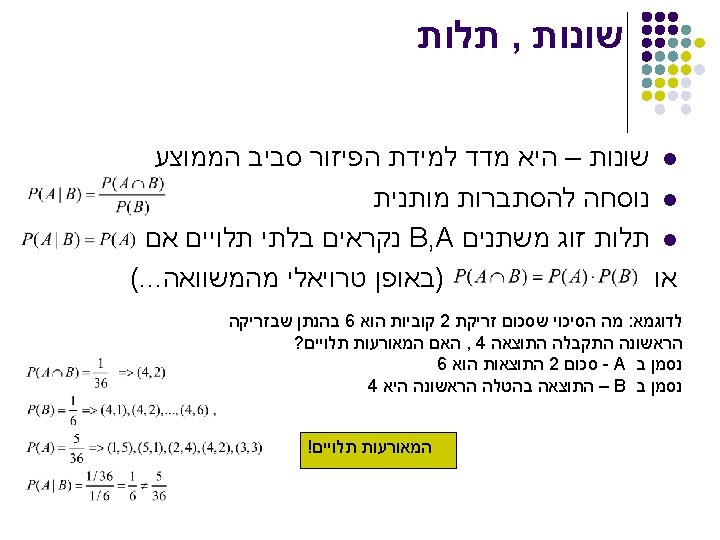
The dimension problem l l l Suppose , we want to calculate the probability to have a hard disease base on N parameters : age , height , weight , blood pressure , country , historical treatments , genetics ext. . We calculate for each sample M feature , if we have N samples we can describe it as Mx. N matrix probably that only few number of features are important - how can we find them?

The dimension problem l l l Some features are not informative Constant feature – the variance of the vector is zero or close to zero , lets say that in our experiments , we check the birth country of the samples , and 98% of them was born in Israel while 2% was born in other country Feature that are linearly dependent on other features like blood pressure and weight Informative features - high variance between groups and low variance in the group

Algebraic Interpretation – 1 D l Given m points in a n dimensional space, for large n, how does one project on to a 1 dimensional space? l Choose a line that fits the data so the points are spread out well along the line

Algebraic Interpretation – 1 D l l l Given m points in a n dimensional space, for large n, how does one project on to a low dimensional space while preserving broad trends in the data and allowing it to be visualized? Formally, minimize sum of squares of distances to the line. Why sum of squares? Because it allows fast minimization, assuming the line passes through 0

Principal Components l l 25 Wavelength 2 All principal components (PCs) start at the origin of the ordinate axes. First PC is direction of maximum variance from origin Subsequent PCs are orthogonal to 1 st PC and describe maximum residual variance 20 15 PC 1 10 5 0 0 5 10 15 20 Wavelength 1 25 30 10 25 30 30 25 Wavelength 2 l 30 20 15 PC 2 10 5 0 0 5 15 20 Wavelength 1

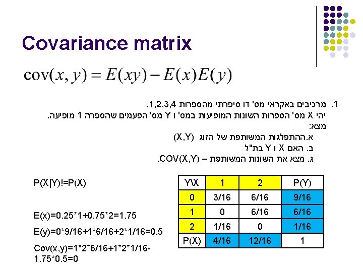
Covariance Matrix l l l Each i, j is the cov(xi, xj) Each i, i is the var(xi) In the previous question V(X)=1*0. 25+4*0. 751. 75*1. 75= V(Y)=1*6/16+4*1/160. 5*0. 5

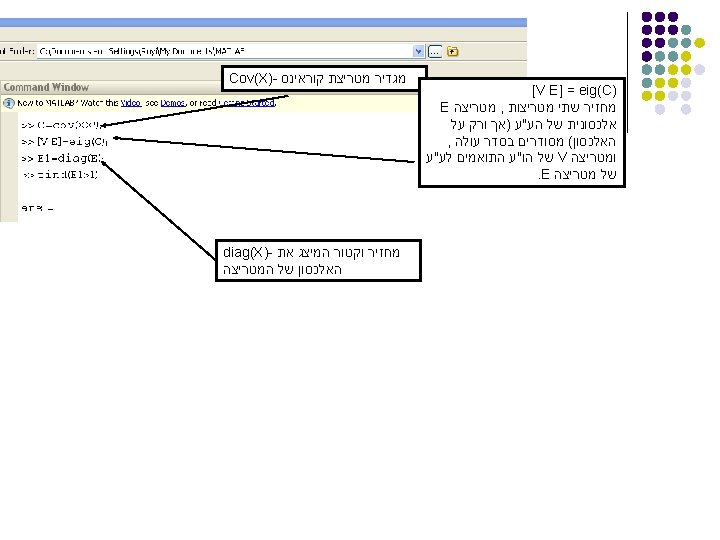
The Algorithm l Step 1: Calculate the Covariance Matrix of the observation matrix. l Step 2: Calculate the eigenvalues and the corresponding eigenvectors. l Step 3: Sort eigenvectors by the magnitude of their eigenvalues. l Step 4: Project the data points on those vectors.

PCA – Step 1: Covariance Matrix C Ø - Data Matrix

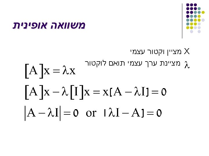
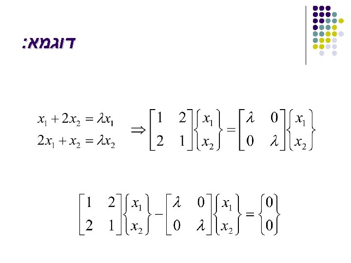
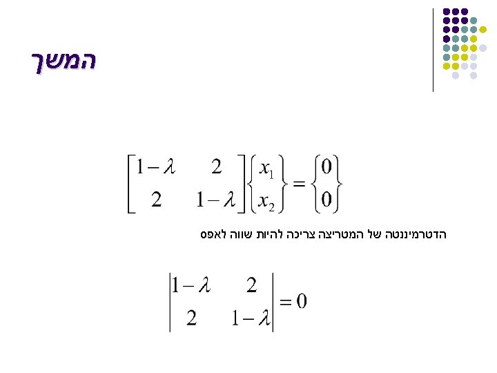
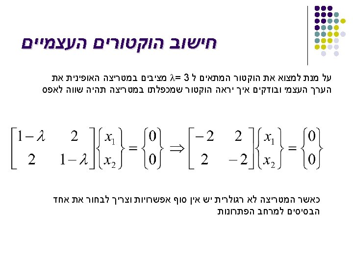
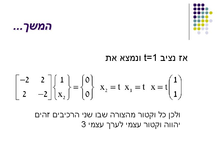
Linear Algebra Review – Eigenvalue and Eigenvector eigenvector l C - a square n n matrix eigenvalue

PCA – Step 3 l Sort eigenvectors by the magnitude of their eigenvalues

PCA – Step 4 l Project the input data onto the principal components. l The new data values are generated for each observation, which are a linear combination as follows: ° ° ° score observation principal component loading (-1 to 1) variable

PCA: General From k original variables: x 1, x 2, . . . , xk: Produce k new variables: y 1, y 2, . . . , yk: y 1 = a 11 x 1 + a 12 x 2 +. . . + a 1 kxk y 2 = a 21 x 1 + a 22 x 2 +. . . + a 2 kxk. . . yk = ak 1 x 1 + ak 2 x 2 +. . . + akkxk such that: yk's are uncorrelated (orthogonal) y 1 explains as much as possible of original variance in data set y 2 explains as much as possible of remaining variance etc.

2 nd Principal Component, y 2 1 st Principal Component, y 1

PCA Scores xi 2 yi, 1 yi, 2 xi 1

PCA Eigenvalues λ 1 λ 2

PCA: Another Explanation From k original variables: x 1, x 2, . . . , xk: Produce k new variables: y 1, y 2, . . . , yk: y 1 = a 11 x 1 + a 12 x 2 +. . . + a 1 kxk y 2 = a 21 x 1 + a 22 x 2 +. . . + a 2 kxk. . . yk = ak 1 x 1 + ak 2 x 2 +. . . + akkxk yk's are Principal Components such that: yk's are uncorrelated (orthogonal) y 1 explains as much as possible of original variance in data set y 2 explains as much as possible of remaining variance etc.

Example from 2005 b Perform pca for the following data sets X=(0, 0), (1, 1), (2, 2), (3, 3), (-1, -1), (-2, -2), (-3, -3) Mean(x)=0