PCA EFA and PA Chong Ho Yu PCA

PCA, EFA, and PA Chong Ho Yu

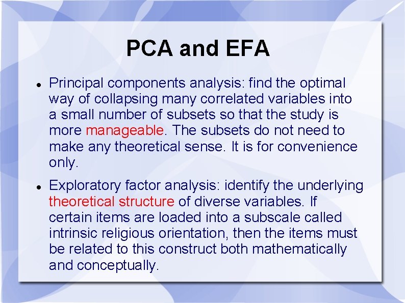
PCA and EFA Principal components analysis: find the optimal way of collapsing many correlated variables into a small number of subsets so that the study is more manageable. The subsets do not need to make any theoretical sense. It is for convenience only. Exploratory factor analysis: identify the underlying theoretical structure of diverse variables. If certain items are loaded into a subscale called intrinsic religious orientation, then the items must be related to this construct both mathematically and conceptually.

Example of PCA: Insurance policy The policy variables (Maitra & Yan): Fire Protection Class Number of Building in Policy Number of Locations in Policy Maximum Building Age Building Coverage Indicator Policy Age

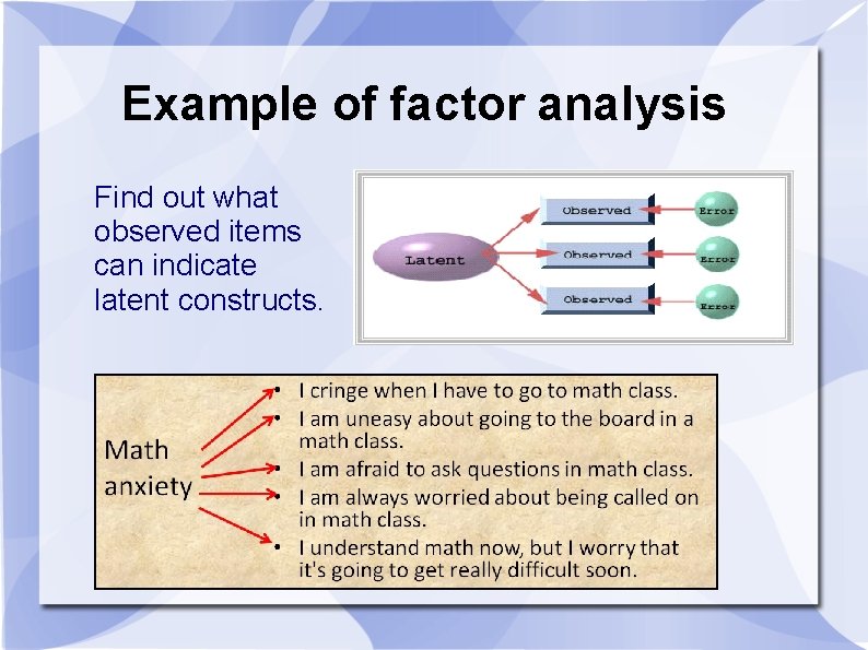
Example of factor analysis Find out what observed items can indicate latent constructs.

Alternatives to PCA and EFA Item response theory (IRT) and Rasch modeling Not covered now; you need to take Psychometrics Yu, C. H. (2020). Objective measurement: How Rasch modeling can simplify and enhance your assessment. In M. S. Khine (Ed. ). Rasch measurement: Applications in quantitative educational research (pp. 47 -73). Singapore: Springer. https: //doi. org/10. 1007/978 -981 -15 -1800 -3_4.

Alternatives to PCA and EFA Yu, C. H. (2019). An Analysis of the relationship between Christian faith and mental wellbeing using item response theory. PEOPLE: International Journal of Social Sciences, 5, 565 -586. DOI: https: //doi. org/10. 20319/pijss. 2019. 53. 565586 Yu, C. H. , Osborn-Popp, S. , Di. Gangi, S. , & Jannasch. Pennell, A. (2007). Assessing unidimensionality: A comparison of Rasch Modeling, Parallel Analysis, and TETRAD. Practical Assessment, Research and Evaluation, 12. Retrieved from http: //pareonline. net/pdf/v 12 n 14. pdf

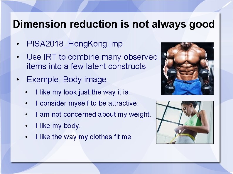
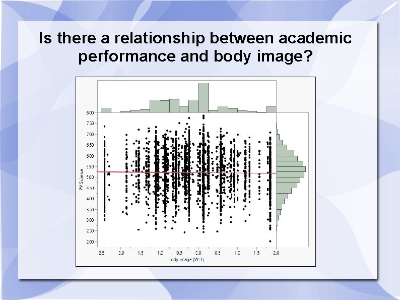
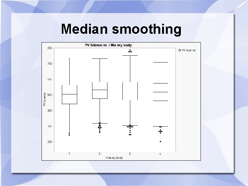
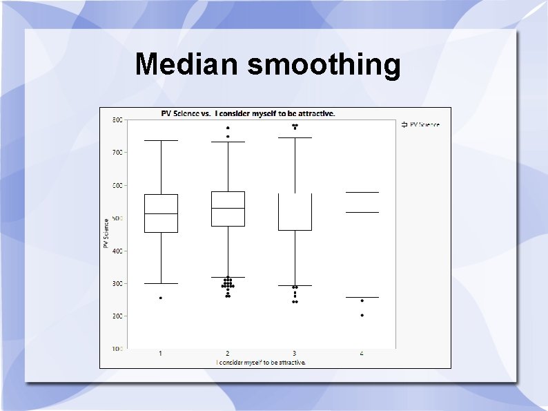
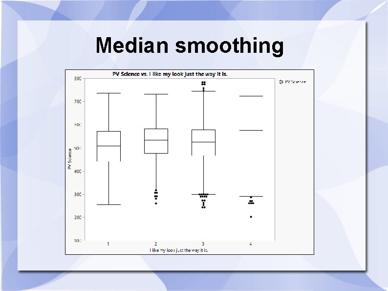
Dimension reduction is not always good • PISA 2018_Hong. Kong. jmp • Use IRT to combine many observed items into a few latent constructs • Example: Body image • I like my look just the way it is. • I consider myself to be attractive. • I am not concerned about my weight. • I like my body. • I like the way my clothes fit me

Is there a relationship between academic performance and body image?

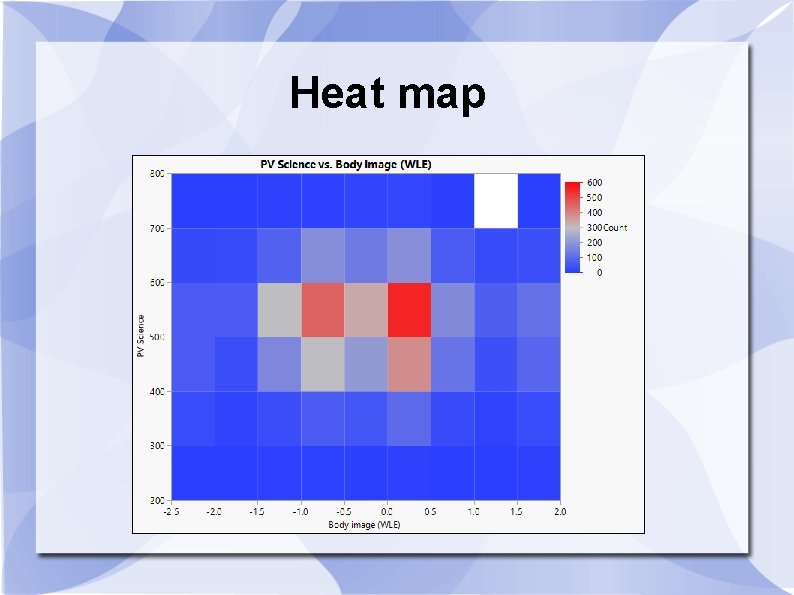
Heat map

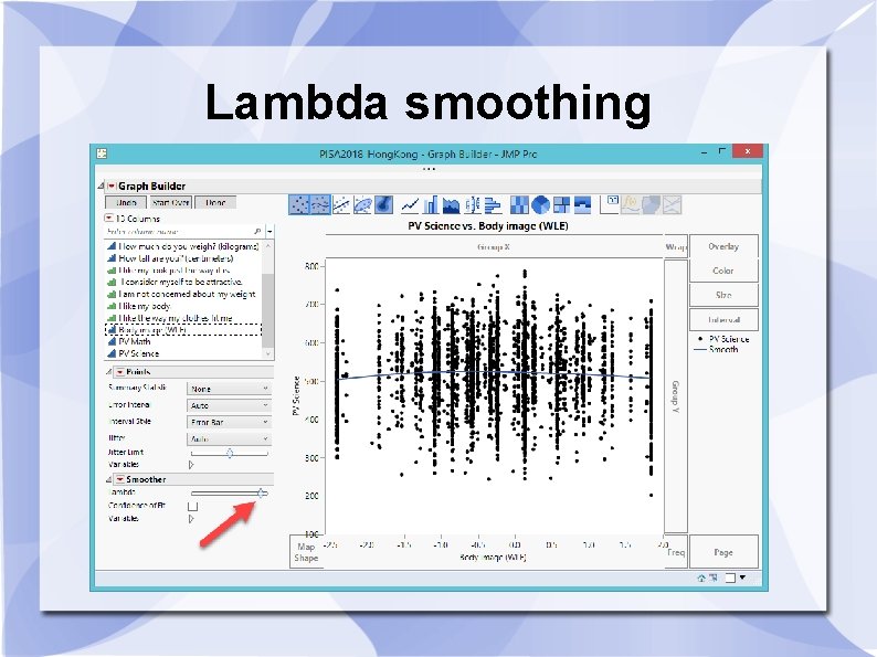
Lambda smoothing

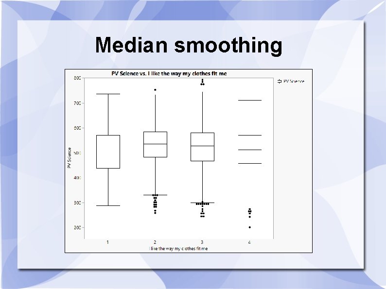
Median smoothing

Median smoothing

Median smoothing

Median smoothing

Lesson from PISA 2018 • When the data set is big, scatterplot with histograms, heat map, lambda smoothing cannot show the relationship between science test performance and the latent construct “body image. ” • When science test score and each item related to body image are examined, a nonlinear relationship is discovered.

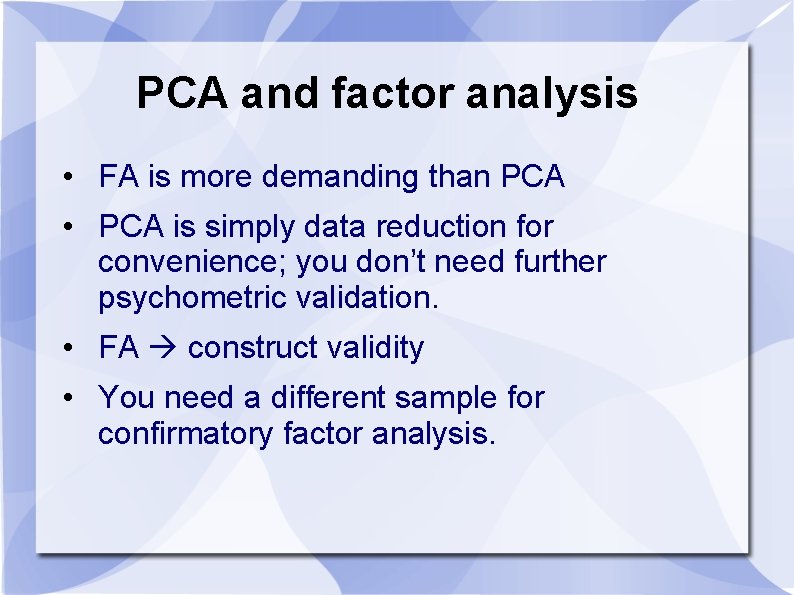
PCA and factor analysis • FA is more demanding than PCA • PCA is simply data reduction for convenience; you don’t need further psychometric validation. • FA construct validity • You need a different sample for confirmatory factor analysis.

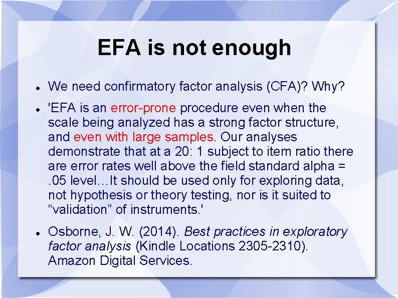
EFA is not enough We need confirmatory factor analysis (CFA)? Why? 'EFA is an error-prone procedure even when the scale being analyzed has a strong factor structure, and even with large samples. Our analyses demonstrate that at a 20: 1 subject to item ratio there are error rates well above the field standard alpha =. 05 level…It should be used only for exploring data, not hypothesis or theory testing, nor is it suited to “validation” of instruments. ' Osborne, J. W. (2014). Best practices in exploratory factor analysis (Kindle Locations 2305 -2310). Amazon Digital Services.

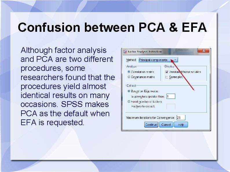
Confusion between PCA & EFA Although factor analysis and PCA are two different procedures, some researchers found that the procedures yield almost identical results on many occasions. SPSS makes PCA as the default when EFA is requested.

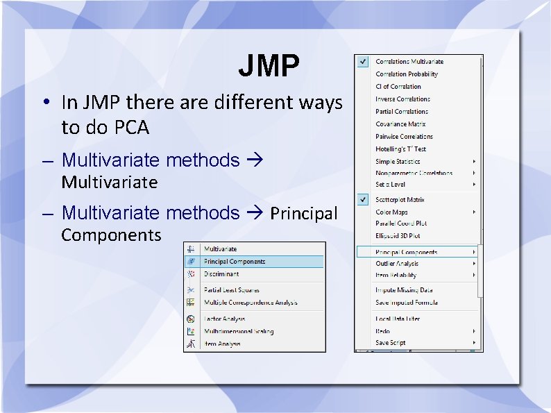
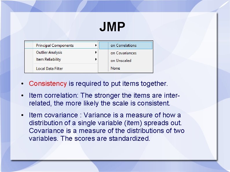
JMP • In JMP there are different ways to do PCA – Multivariate methods Multivariate – Multivariate methods Principal Components

JMP • Consistency is required to put items together. • Item correlation: The stronger the items are interrelated, the more likely the scale is consistent. • Item covariance : Variance is a measure of how a distribution of a single variable (item) spreads out. Covariance is a measure of the distributions of two variables. The scores are standardized.

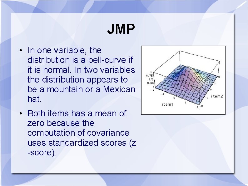
JMP • In one variable, the distribution is a bell-curve if it is normal. In two variables the distribution appears to be a mountain or a Mexican hat. • Both items has a mean of zero because the computation of covariance uses standardized scores (z -score).

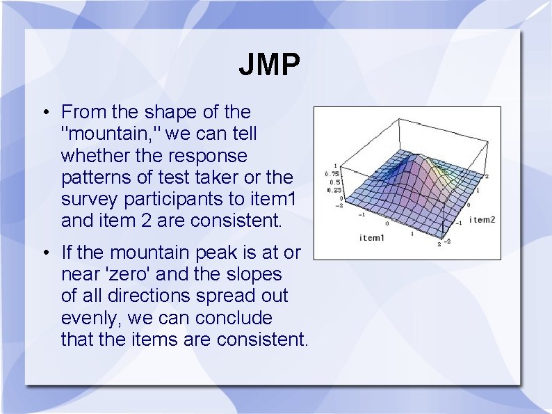
JMP • From the shape of the "mountain, " we can tell whether the response patterns of test taker or the survey participants to item 1 and item 2 are consistent. • If the mountain peak is at or near 'zero' and the slopes of all directions spread out evenly, we can conclude that the items are consistent.

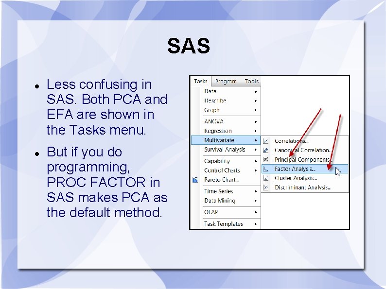
SAS Less confusing in SAS. Both PCA and EFA are shown in the Tasks menu. But if you do programming, PROC FACTOR in SAS makes PCA as the default method.

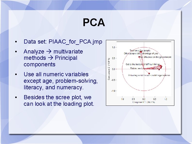
PCA • Data set: PIAAC_for_PCA. jmp • Analyze multivariate methods Principal components • Use all numeric variables except age, problem-solving, literacy, and numeracy. • Besides the scree plot, we can look at the loading plot.

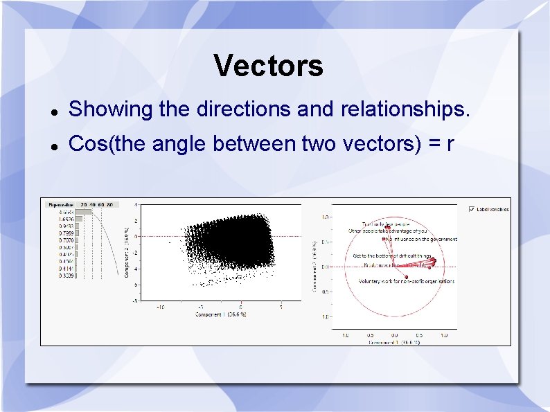
Vectors Showing the directions and relationships. Cos(the angle between two vectors) = r

Vector • A mathematical object with a numeric value is called a scalar. • A mathematical object that has both a numeric value and a direction is called a vector. • If I just tell you to drive 10 miles to reach my home, this instruction is definitely useless. I must say something like, "From Claremont drive 10 miles West to Azusa. "

Vector • Vector-based graphics: the image is defined by the relationships among vectors instead of the composition of pixels. • For example, to construct a shape, the software stores the information like "Start from point A, draw a straight line at 45 degrees, stop at 10 units, draw another line at 35 degrees. . . "

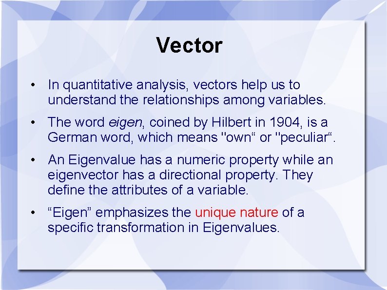
Vector • In quantitative analysis, vectors help us to understand the relationships among variables. • The word eigen, coined by Hilbert in 1904, is a German word, which means "own“ or "peculiar“. • An Eigenvalue has a numeric property while an eigenvector has a directional property. They define the attributes of a variable. • “Eigen” emphasizes the unique nature of a specific transformation in Eigenvalues.

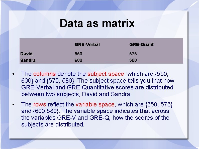
Data as matrix David Sandra GRE-Verbal GRE-Quant 550 600 575 580 • The columns denote the subject space, which are {550, 600} and {575, 580}. The subject space tells you that how GRE-Verbal and GRE-Quantitative scores are distributed between two subjects, David and Sandra. • The rows reflect the variable space, which are {550, 575} and {600, 580}. The variable space indicates that across the variables GRE-V and GRE-Q, how the scores of the subjects are distributed.

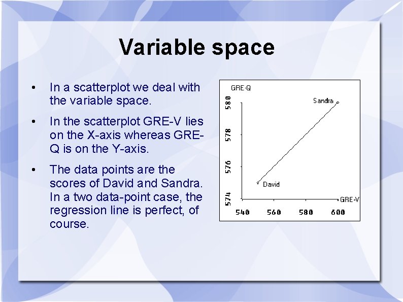
Variable space • In a scatterplot we deal with the variable space. • In the scatterplot GRE-V lies on the X-axis whereas GREQ is on the Y-axis. • The data points are the scores of David and Sandra. In a two data-point case, the regression line is perfect, of course.

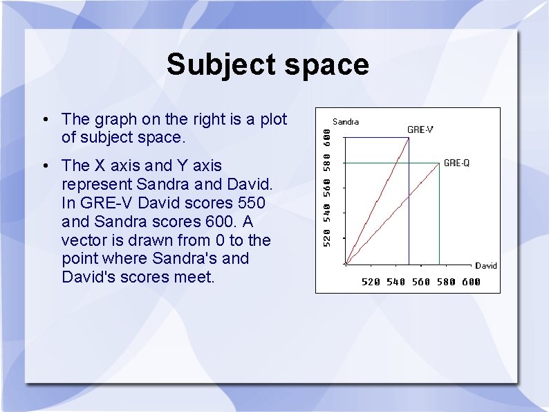
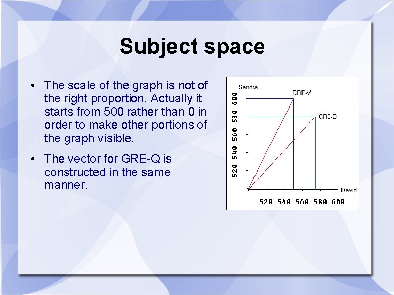
Subject space • The graph on the right is a plot of subject space. • The X axis and Y axis represent Sandra and David. In GRE-V David scores 550 and Sandra scores 600. A vector is drawn from 0 to the point where Sandra's and David's scores meet.

Subject space • The scale of the graph is not of the right proportion. Actually it starts from 500 rather than 0 in order to make other portions of the graph visible. • The vector for GRE-Q is constructed in the same manner.

Hyperspace • When subject space and variable space are combined, we call it the hyperspace. • In reality, a research project always involves more than two variables and two subjects. • In a multi-dimensional hyperspace, the vectors in the subject space can be combined to form an eigenvector, which depicts the Eigenvalue. • The longer the length of the eigenvector is, the higher the Eigenvalue is and the more variance it can explain.

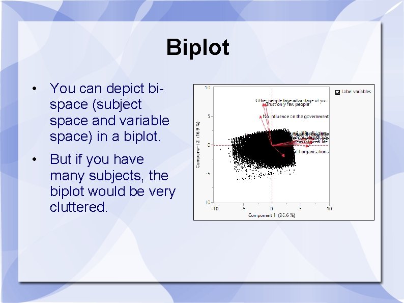
Biplot • You can depict bispace (subject space and variable space) in a biplot. • But if you have many subjects, the biplot would be very cluttered.

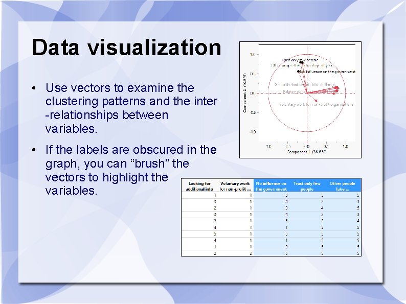
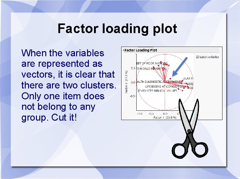
Data visualization • Use vectors to examine the clustering patterns and the inter -relationships between variables. • If the labels are obscured in the graph, you can “brush” the vectors to highlight the variables.

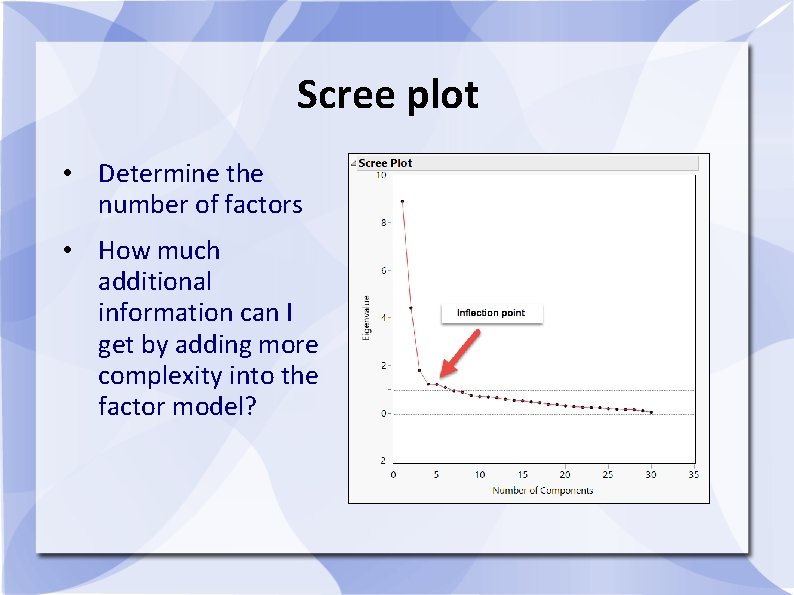
Scree plot • Determine the number of factors • How much additional information can I get by adding more complexity into the factor model?

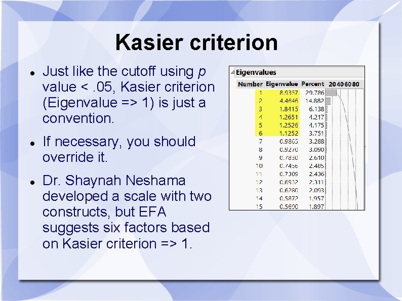
Kasier criterion Just like the cutoff using p value <. 05, Kasier criterion (Eigenvalue => 1) is just a convention. If necessary, you should override it. Dr. Shaynah Neshama developed a scale with two constructs, but EFA suggests six factors based on Kasier criterion => 1.

Factor loading plot When the variables are represented as vectors, it is clear that there are two clusters. Only one item does not belong to any group. Cut it!

Assignment 9. 1 • Data set: PIAAC_for _PCA. jmp • Run a PCA with problem-solving, literacy, and numeracy. • Examine the loading plot • Can we put all three test scores together as a composite score? Are all vectors close to each other?

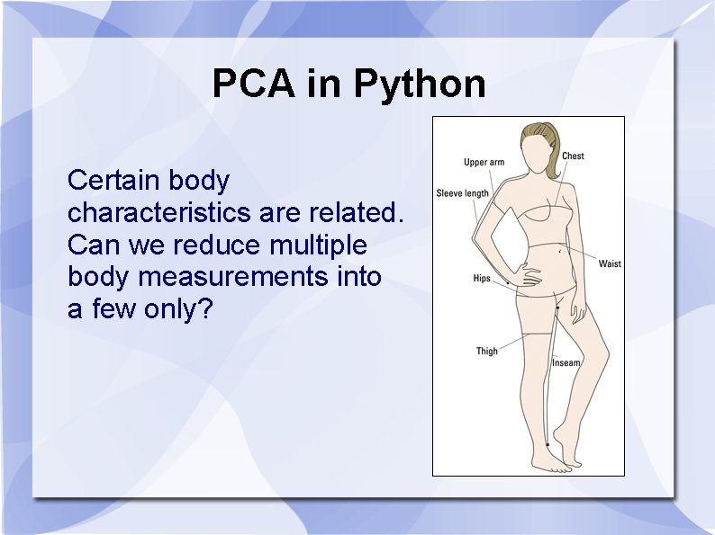
PCA in Python Certain body characteristics are related. Can we reduce multiple body measurements into a few only?

PCA in Python • Download the files “python_PCA. txt” and “body_measurement. xlsx” from the folder “Python_files” in Unit 9. • Open a new Python interpreter. • Run the Python codes chunk by chunk.

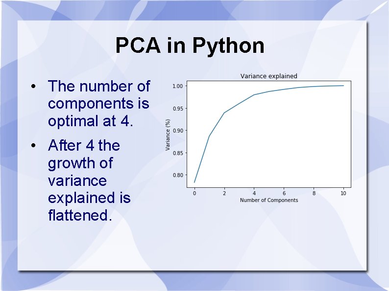
PCA in Python • The number of components is optimal at 4. • After 4 the growth of variance explained is flattened.

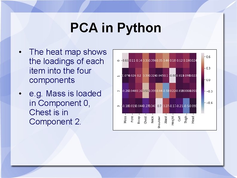
PCA in Python • The heat map shows the loadings of each item into the four components • e. g. Mass is loaded in Component 0, Chest is in Component 2.

Various criteria Kasier criterion The scree plot Parallel analysis Many studies had verified that by far PA is the most accurate method (Buja & Eyubuglu, 1992; Glorfeld, 1995; Horn, 1965; Hubbard & Allen, 1987; Humphreys & Montanelli, 1975; Velicer et al. , 2000; Zwick & Velicer, 1986).

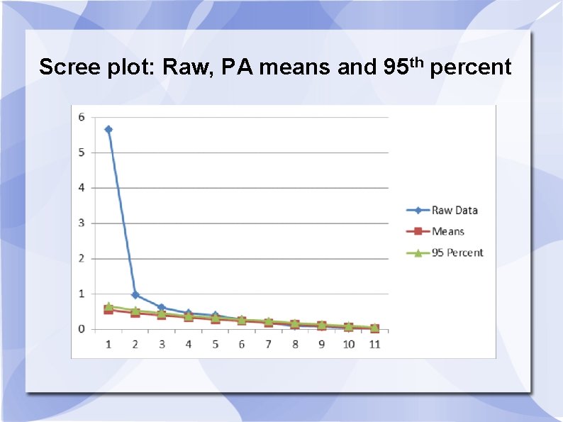
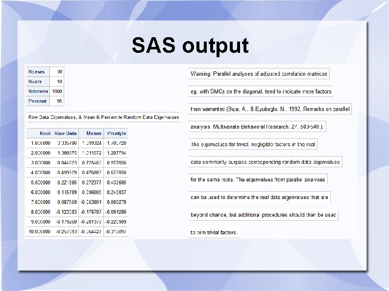
Parallel Analysis: Resampling The logic of parallel analysis resembles that of resampling: the number of factors extracted should have eigenvalues greater than those in a random matrix. The algorithm generates a set of random data correlation matrices by bootstrapping the data set (resampling with replacement), and then the average eigenvalues and the 95 th percentile eigenvalues are computed.

PA: Resampling The observed eigenvalues are compared against the resampled eigenvalues, and only factors with observed eigenvalues greater than those from re-sampling are retained. The resampled result functions as an empirical sampling distribution, in which the observed is compared against. The rationale of using the 95 th percentile of the resampled data eigenvalues is that this is analogous to setting the value of alpha to. 05 in hypothesis testing (Cho, Li, & Bandalos, 2009).

Underfactoring vs. overfactoring Parallel analysis can be used with PCA or EFA. Which one should be used? PA with PCA tends to under-factoring (extract fewer factors than what it should be). PA with EFA tends to over-factoring (extract more factors than what it should be).

Underfactoring vs. overfactoring Under-factoring is a more serious problem than over-factoring. In the former scenario the researcher totally misses some information. In the latter the result may include some meaningless factors (Crawford, Green, Levy, Lo, Scott, Svetina, & Thompson, 2010), but the researcher can always trim the redundant factors later.

Underfactoring vs. overfactoring It is better to over-prepare than under-prepare. Consider this analogy: I travel with 3 -4 cameras. If I don't need the backup, it is fine. But if I have one camera only and it malfunctions, there is nothing I can do! If your coauthor sends you a 50 -page draft, you can remove the redundant information. If she sends you two pages only, there is nothing you can do!

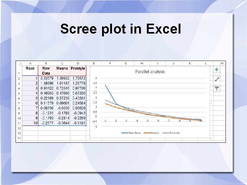
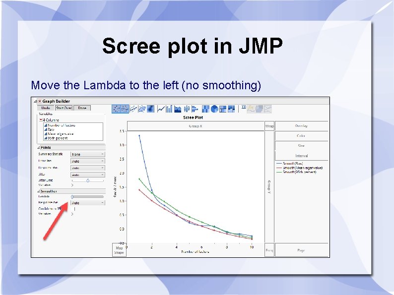
Scree plot: Raw, PA means and 95 th percent

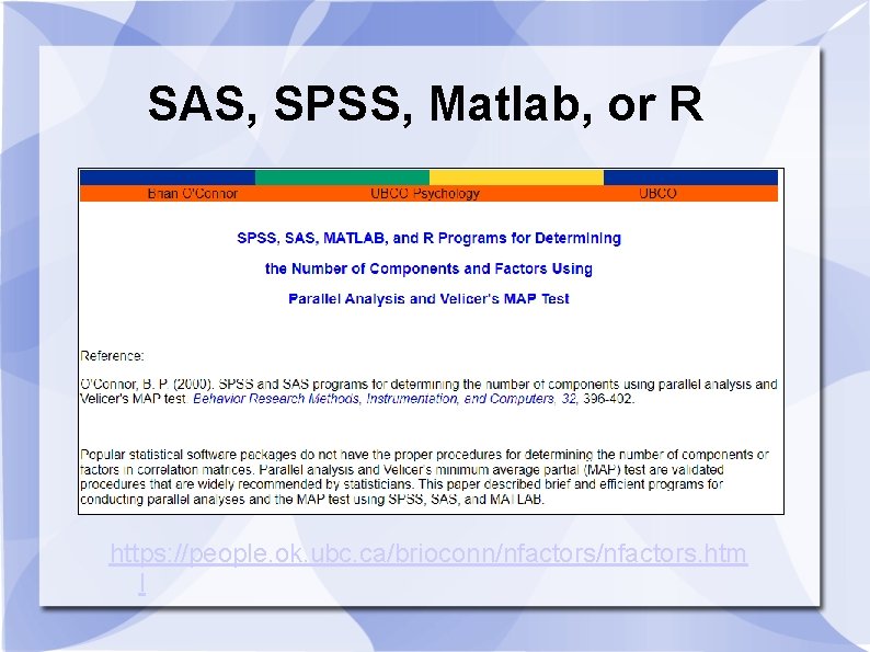
SAS, SPSS, Matlab, or R https: //people. ok. ubc. ca/brioconn/nfactors. htm l

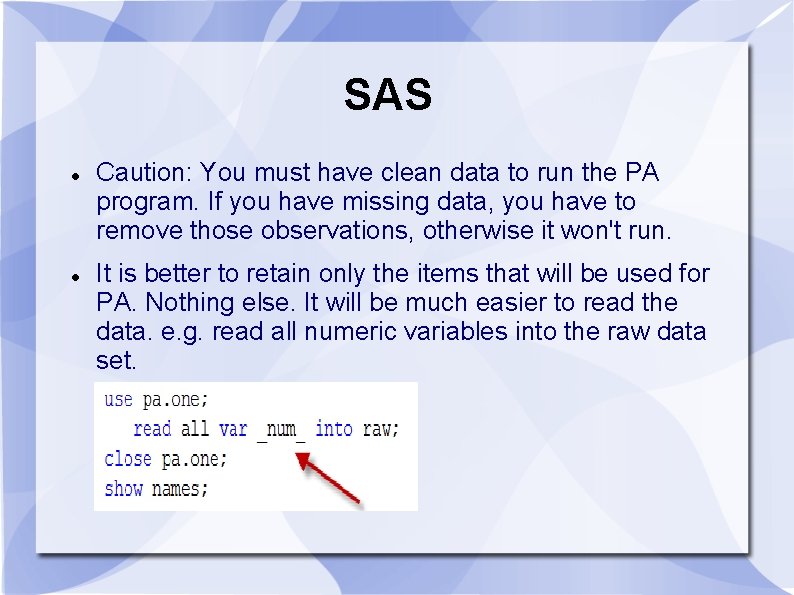
SAS Caution: You must have clean data to run the PA program. If you have missing data, you have to remove those observations, otherwise it won't run. It is better to retain only the items that will be used for PA. Nothing else. It will be much easier to read the data. e. g. read all numeric variables into the raw data set.

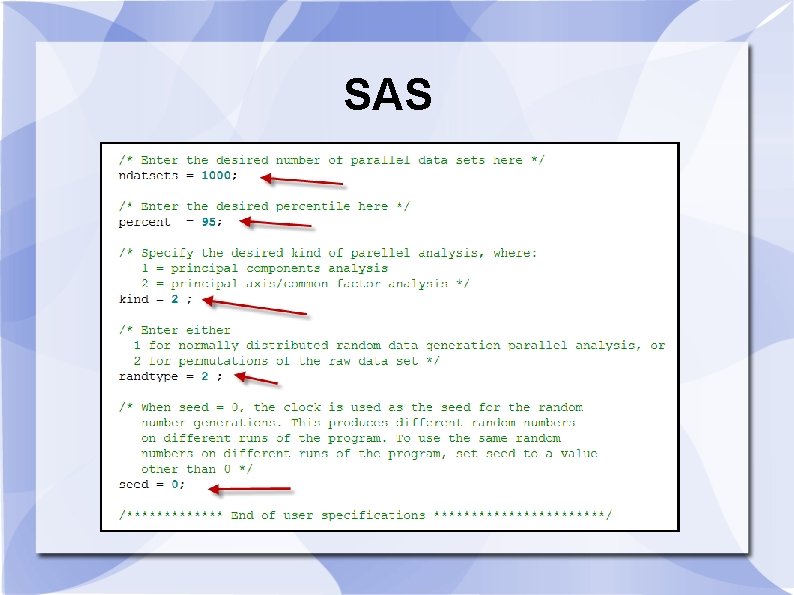
SAS

SAS output

Scree plot in Excel

Scree plot in JMP Move the Lambda to the left (no smoothing)

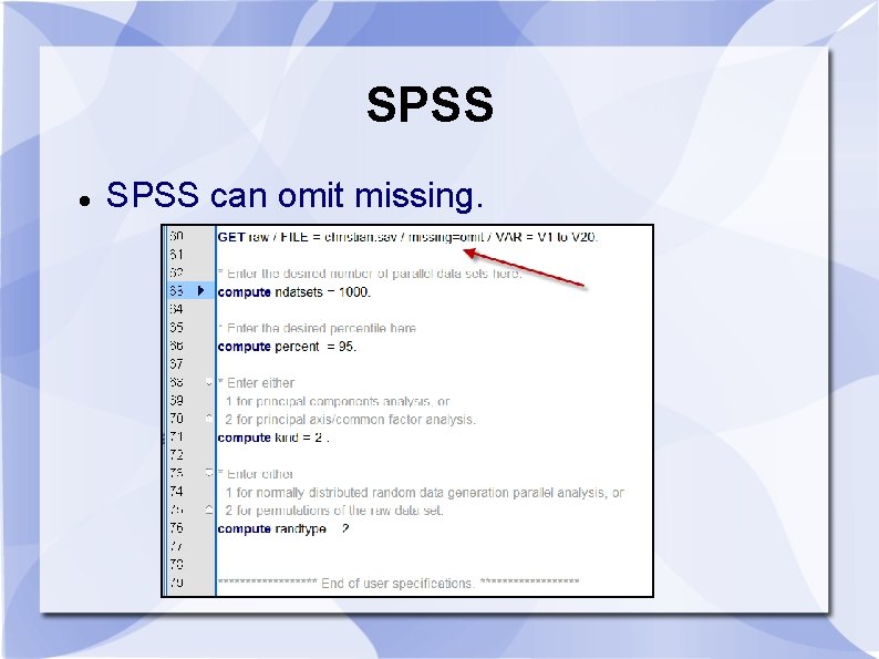
SPSS can omit missing.

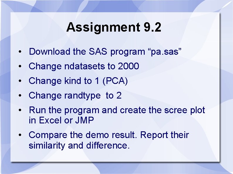
Assignment 9. 2 • Download the SAS program “pa. sas” • Change ndatasets to 2000 • Change kind to 1 (PCA) • Change randtype to 2 • Run the program and create the scree plot in Excel or JMP • Compare the demo result. Report their similarity and difference.