Principal Component Analysis What is it Principal Component

- Slides: 29

Principal Component Analysis • What is it? • Principal Component Analysis (PCA) is a standard tool in multivariate analysis for examining multidimensional data • To reveal patterns between objects that would not be apparent in a univariate analysis • What is the goal of PCA? • PCA reduces a correlated dataset (values of variables {x 1, x 2, …, xp}) to a dataset containing fewer new variables by axis rotation • The new variables are linear combinations of the original ones and are uncorrelated • The PCs are the new variables (or axes) which summarize several of the original variables • If nonzero correlation exists among the variables of the data set, then it is possible to determine a more compact description of the data, which amounts to finding the dominant modes in the data.

How does it work? • PCA can explain most of the variability of the original dataset in a few new variables (if data are well correlated) • Correlation introduces redundancy (if two variables are perfectly correlated, then one of them is redundant because if we know x, we know y) • PCA exploits this redundancy in multivariate data to pick out patterns and relationships in the variables and reduce the dimensionality of the dataset without significant loss of information

What do we use it for? • Types of data we can use PCA on: • Basically anything! • Usually we have multiple variables (may be different locations of the same variables, or different variables) and samples or replicates of these variables (e. g. samples taken at different times, or data relating to different subjects or locations) • Very useful in the geosciences where data are generally well correlated (across variables, across space) • What can it be used for? • Exploratory data analysis • Detection of outliers • Identification of clusters (grouping, regionalization) • Reduction of variables (data pre-processing, multivariate modeling) • Data compression (lossy!) • Analysis of variability in space and time • New interpretation of the data (in terms of the main components of variability) • Forecasting (finding relationships between variables)

Some Examples from the Literature • Geosciences in general • Rock type identification • Remote sensing retrievals • Classification of land use • Hydrology, water quality and ecology • Regionalization (e. g. drought and flood regimes) • Analysis of water quality and relationships with hydrology • Relationships between species richness with morphological and hydrological parameters (lake size, land use, hydraulic residence time) • Relationships between hydrology/soils and vegetation patterns • Contamination source identification • Atmospheric science and climate analysis • Weather typing and classification • Identification of major modes of variability • Teleconnection patterns • The Hockey stick plot of global temperature record (example of perceived misuse of PCA – actually NOT!) • Others • Bioinformatics • Gene expressions analysis • Image processing and pattern recognition • Data compression

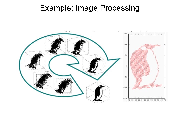
Example: Image Processing

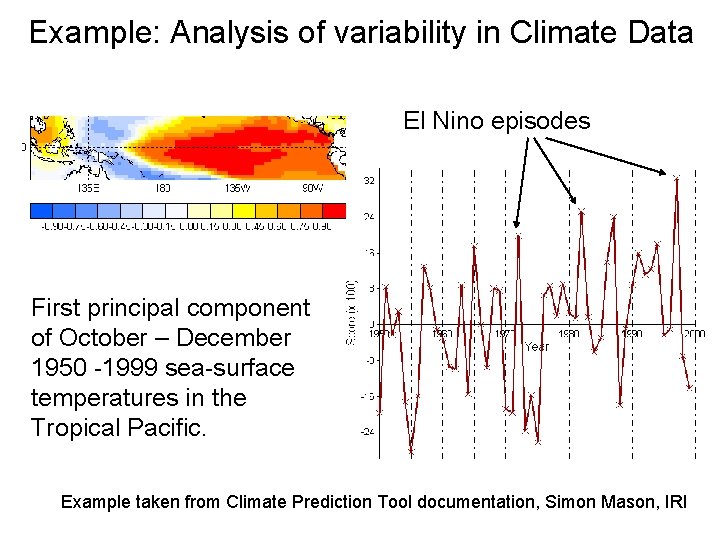
Example: Analysis of variability in Climate Data El Nino episodes First principal component of October – December 1950 -1999 sea-surface temperatures in the Tropical Pacific. Example taken from Climate Prediction Tool documentation, Simon Mason, IRI

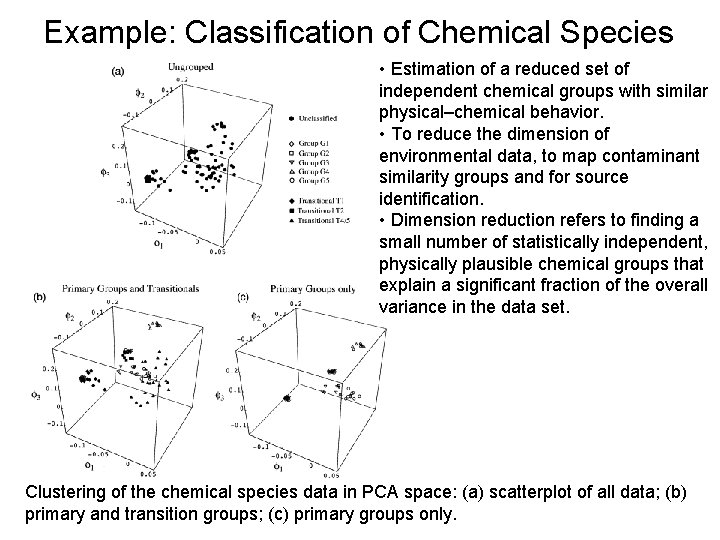
Example: Classification of Chemical Species • Estimation of a reduced set of independent chemical groups with similar physical–chemical behavior. • To reduce the dimension of environmental data, to map contaminant similarity groups and for source identification. • Dimension reduction refers to finding a small number of statistically independent, physically plausible chemical groups that explain a significant fraction of the overall variance in the data set. Clustering of the chemical species data in PCA space: (a) scatterplot of all data; (b) primary and transition groups; (c) primary groups only.

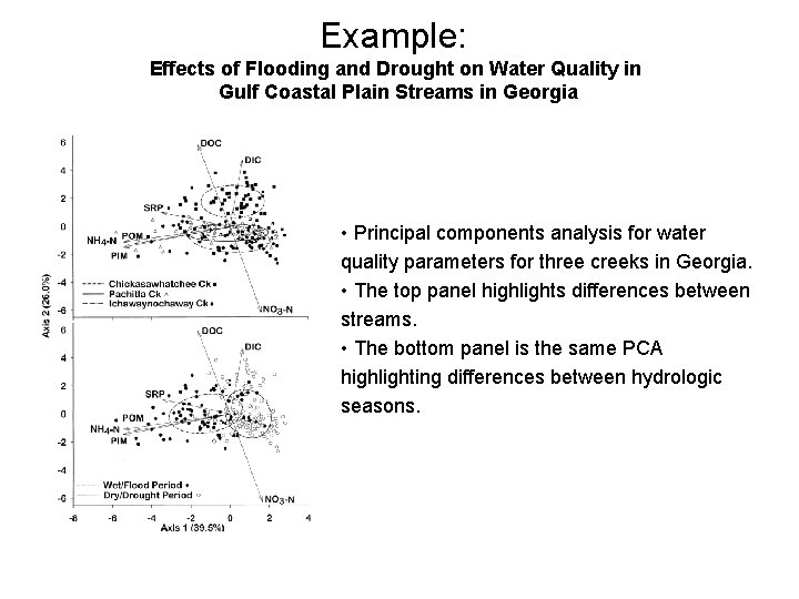
Example: Effects of Flooding and Drought on Water Quality in Gulf Coastal Plain Streams in Georgia • Principal components analysis for water quality parameters for three creeks in Georgia. • The top panel highlights differences between streams. • The bottom panel is the same PCA highlighting differences between hydrologic seasons.

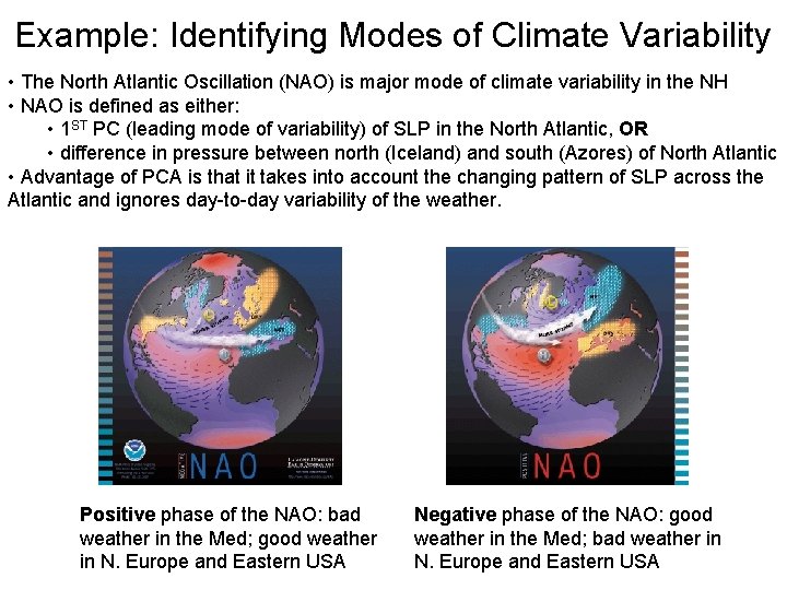
Example: Identifying Modes of Climate Variability • The North Atlantic Oscillation (NAO) is major mode of climate variability in the NH • NAO is defined as either: • 1 ST PC (leading mode of variability) of SLP in the North Atlantic, OR • difference in pressure between north (Iceland) and south (Azores) of North Atlantic • Advantage of PCA is that it takes into account the changing pattern of SLP across the Atlantic and ignores day-to-day variability of the weather. Positive phase of the NAO: bad weather in the Med; good weather in N. Europe and Eastern USA Negative phase of the NAO: good weather in the Med; bad weather in N. Europe and Eastern USA

Example: Global soil moisture variability How do we analyze a global dataset of soil moisture with 50 -yrs of data at 15000 grid points? • How does it vary in time and space? • What are the main modes of variability? • Can we relate these to physical phenomena?

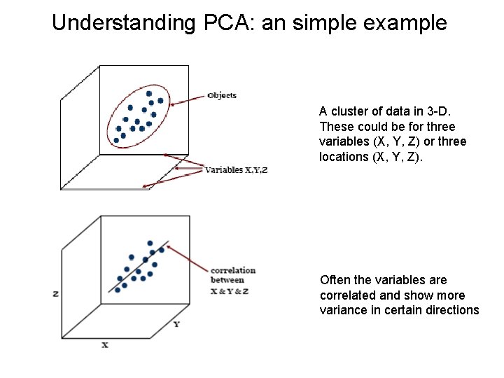
Understanding PCA: an simple example A cluster of data in 3 -D. These could be for three variables (X, Y, Z) or three locations (X, Y, Z). Often the variables are correlated and show more variance in certain directions

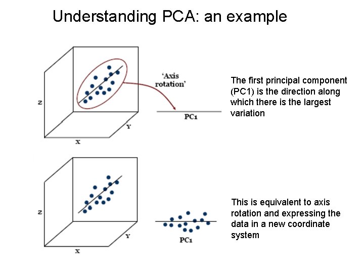
Understanding PCA: an example The first principal component (PC 1) is the direction along which there is the largest variation This is equivalent to axis rotation and expressing the data in a new coordinate system

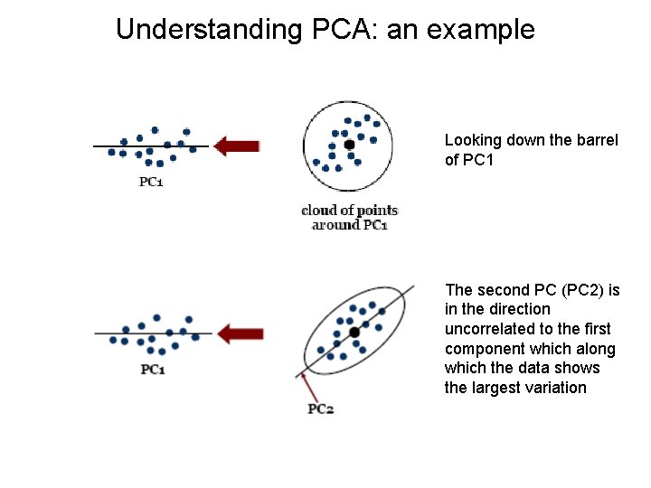
Understanding PCA: an example Looking down the barrel of PC 1 The second PC (PC 2) is in the direction uncorrelated to the first component which along which the data shows the largest variation

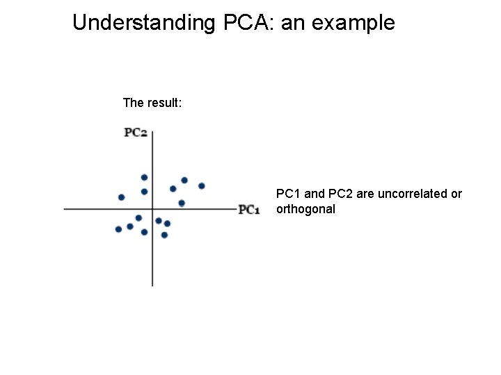
Understanding PCA: an example The result: PC 1 and PC 2 are uncorrelated or orthogonal

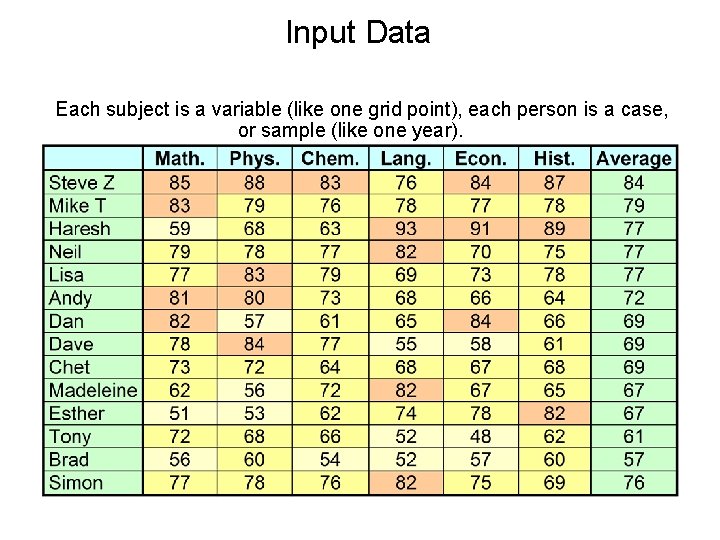
Understanding PCA: a REAL example • Given set of exam scores of a group of 14 people, how can we best summarize the scores? • One objective of summarizing the scores would be to distinguish the good students from the bad students. • Principal components are ideal for obtaining such summaries, but they can also provide other informative summaries … Example taken from Climate Prediction Tool documentation, Simon Mason, IRI

Input Data Each subject is a variable (like one grid point), each person is a case, or sample (like one year).

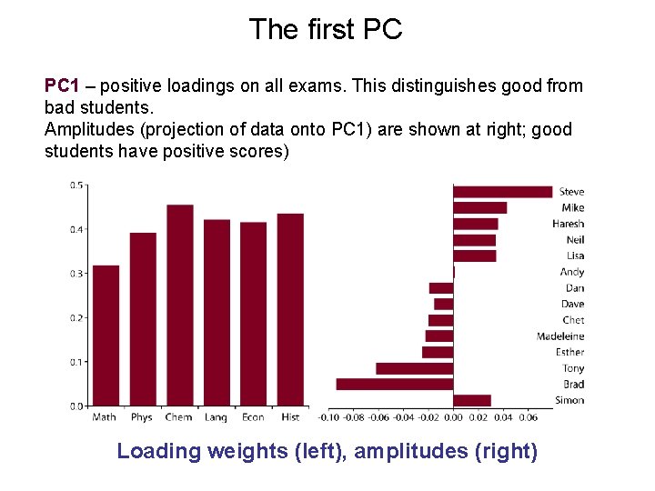
The first PC PC 1 – positive loadings on all exams. This distinguishes good from bad students. Amplitudes (projection of data onto PC 1) are shown at right; good students have positive scores) Loading weights (left), amplitudes (right)

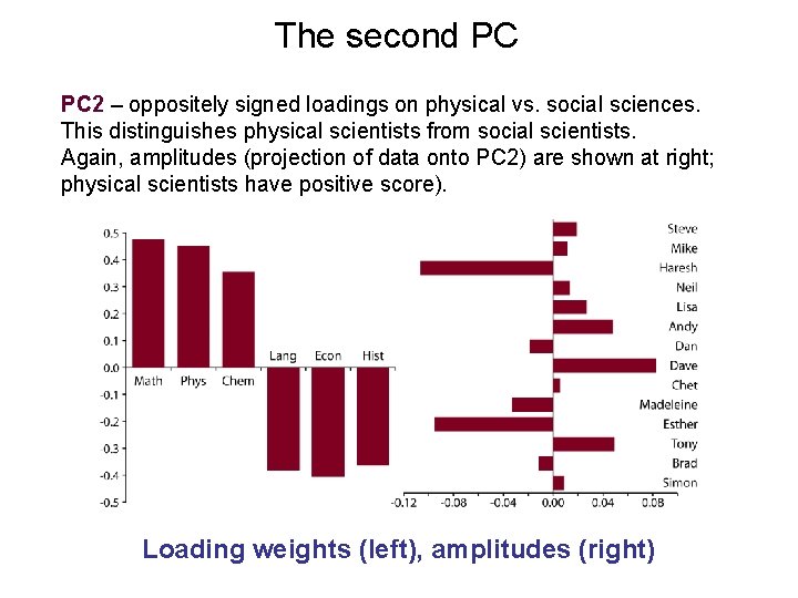
The second PC PC 2 – oppositely signed loadings on physical vs. social sciences. This distinguishes physical scientists from social scientists. Again, amplitudes (projection of data onto PC 2) are shown at right; physical scientists have positive score). Loading weights (left), amplitudes (right)

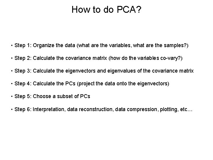
How to do PCA? • Step 1: Organize the data (what are the variables, what are the samples? ) • Step 2: Calculate the covariance matrix (how do the variables co-vary? ) • Step 3: Calculate the eigenvectors and eigenvalues of the covariance matrix • Step 4: Calculate the PCs (project the data onto the eigenvectors) • Step 5: Choose a subset of PCs • Step 6: Interpretation, data reconstruction, data compression, plotting, etc…

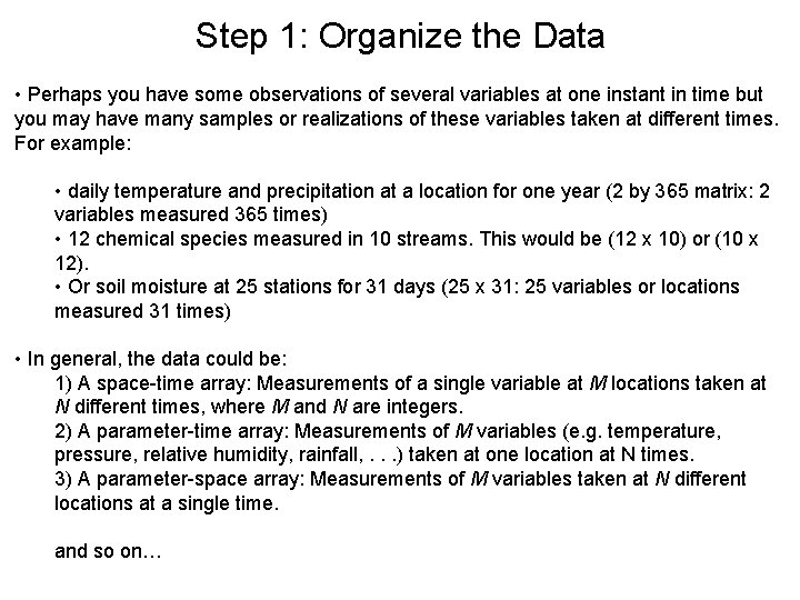
Step 1: Organize the Data • Perhaps you have some observations of several variables at one instant in time but you may have many samples or realizations of these variables taken at different times. For example: • daily temperature and precipitation at a location for one year (2 by 365 matrix: 2 variables measured 365 times) • 12 chemical species measured in 10 streams. This would be (12 x 10) or (10 x 12). • Or soil moisture at 25 stations for 31 days (25 x 31: 25 variables or locations measured 31 times) • In general, the data could be: 1) A space-time array: Measurements of a single variable at M locations taken at N different times, where M and N are integers. 2) A parameter-time array: Measurements of M variables (e. g. temperature, pressure, relative humidity, rainfall, . . . ) taken at one location at N times. 3) A parameter-space array: Measurements of M variables taken at N different locations at a single time. and so on…

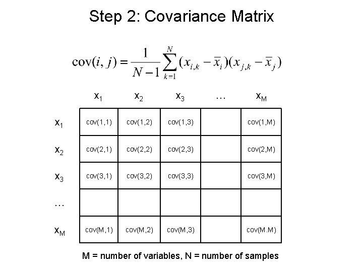
Step 2: Covariance Matrix x 1 x 2 x 3 … x. M x 1 cov(1, 1) cov(1, 2) cov(1, 3) cov(1, M) x 2 cov(2, 1) cov(2, 2) cov(2, 3) cov(2, M) x 3 cov(3, 1) cov(3, 2) cov(3, 3) cov(3, M) cov(M, 1) cov(M, 2) cov(M, 3) cov(M. M) … x. M M = number of variables, N = number of samples

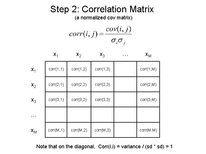
Step 2: Correlation Matrix (a normalized cov matrix) x 1 x 2 x 3 … x. M x 1 corr(1, 1) corr(1, 2) corr(1, 3) corr(1, M) x 2 corr(2, 1) corr(2, 2) corr(2, 3) corr(2, M) x 3 corr(3, 1) corr(3, 2) corr(3, 3) corr(3, M) corr(M, 1) corr(M, 2) corr(M, 3) corr(M. M) … x. M Note that on the diagonal, Corr(i, i) = variance / (sd * sd) = 1

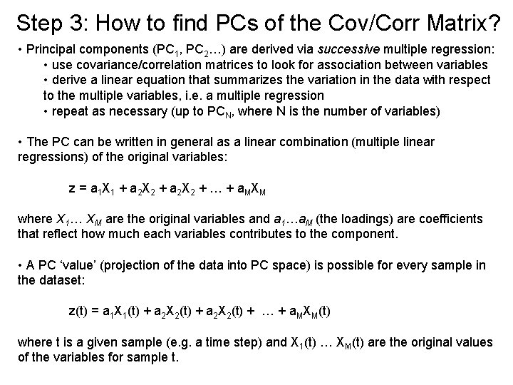
Step 3: How to find PCs of the Cov/Corr Matrix? • Principal components (PC 1, PC 2…) are derived via successive multiple regression: • use covariance/correlation matrices to look for association between variables • derive a linear equation that summarizes the variation in the data with respect to the multiple variables, i. e. a multiple regression • repeat as necessary (up to PCN, where N is the number of variables) • The PC can be written in general as a linear combination (multiple linear regressions) of the original variables: z = a 1 X 1 + a 2 X 2 + … + a. MXM where X 1… XM are the original variables and a 1…a. M (the loadings) are coefficients that reflect how much each variables contributes to the component. • A PC ‘value’ (projection of the data into PC space) is possible for every sample in the dataset: z(t) = a 1 X 1(t) + a 2 X 2(t) + … + a. MXM(t) where t is a given sample (e. g. a time step) and X 1(t) … XM(t) are the original values of the variables for sample t.

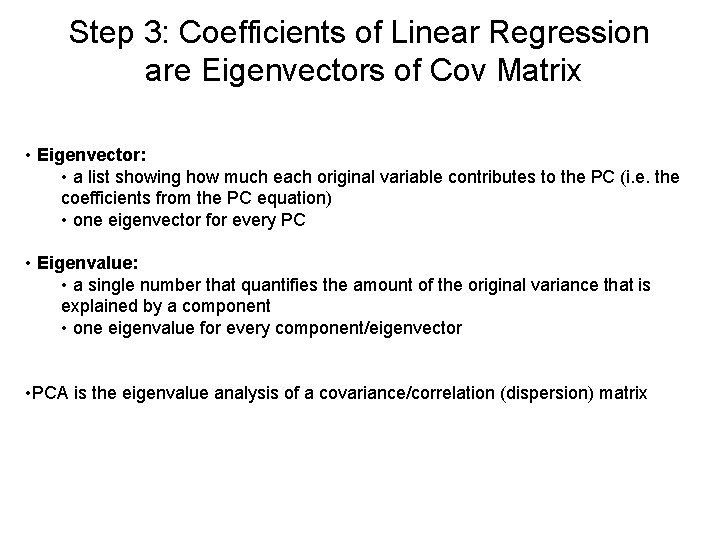
Step 3: Coefficients of Linear Regression are Eigenvectors of Cov Matrix • Eigenvector: • a list showing how much each original variable contributes to the PC (i. e. the coefficients from the PC equation) • one eigenvector for every PC • Eigenvalue: • a single number that quantifies the amount of the original variance that is explained by a component • one eigenvalue for every component/eigenvector • PCA is the eigenvalue analysis of a covariance/correlation (dispersion) matrix

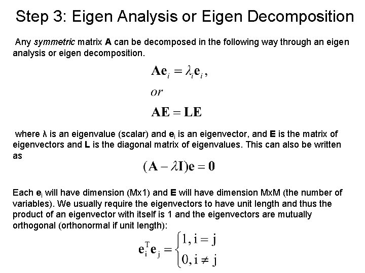
Step 3: Eigen Analysis or Eigen Decomposition Any symmetric matrix A can be decomposed in the following way through an eigen analysis or eigen decomposition. where λ is an eigenvalue (scalar) and ei is an eigenvector, and E is the matrix of eigenvectors and L is the diagonal matrix of eigenvalues. This can also be written as Each ei will have dimension (Mx 1) and E will have dimension Mx. M (the number of variables). We usually require the eigenvectors to have unit length and thus the product of an eigenvector with itself is 1 and the eigenvectors are mutually orthogonal (orthonormal if unit length):

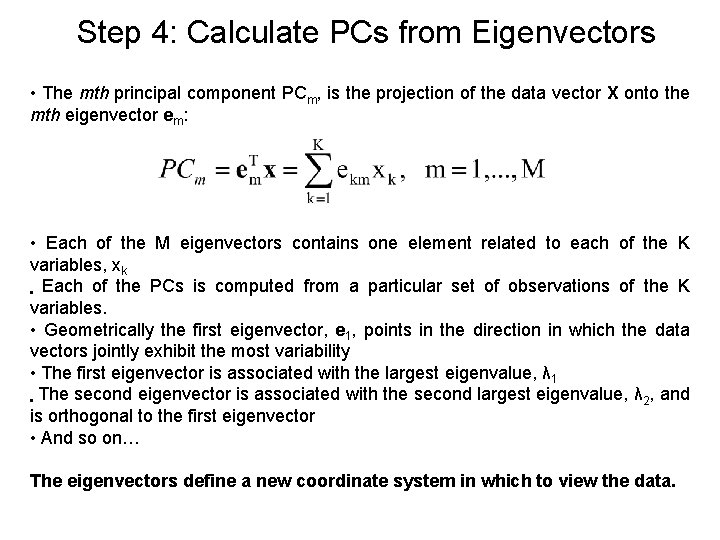
Step 4: Calculate PCs from Eigenvectors • The mth principal component PCm, is the projection of the data vector X onto the mth eigenvector em: • Each of the M eigenvectors contains one element related to each of the K variables, xk • Each of the PCs is computed from a particular set of observations of the K variables. • Geometrically the first eigenvector, e 1, points in the direction in which the data vectors jointly exhibit the most variability • The first eigenvector is associated with the largest eigenvalue, λ 1 • The second eigenvector is associated with the second largest eigenvalue, λ 2, and is orthogonal to the first eigenvector • And so on… The eigenvectors define a new coordinate system in which to view the data.

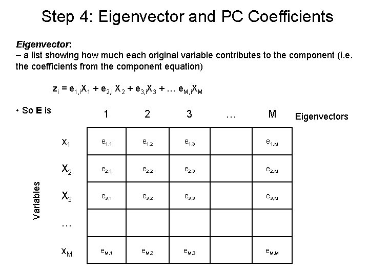
Step 4: Eigenvector and PC Coefficients Eigenvector: – a list showing how much each original variable contributes to the component (i. e. the coefficients from the component equation) zi = e 1, i. X 1 + e 2, i X 2 + e 3, i. X 3 + … e. M, i. XM Variables • So E is 1 2 3 … M x 1 e 1, 2 e 1, 3 e 1, M X 2 e 2, 1 e 2, 2 e 2, 3 e 2, M X 3 e 3, 1 e 3, 2 e 3, 3 e 3, M e. M, 1 e. M, 2 e. M, 3 e. M, M … x. M Eigenvectors

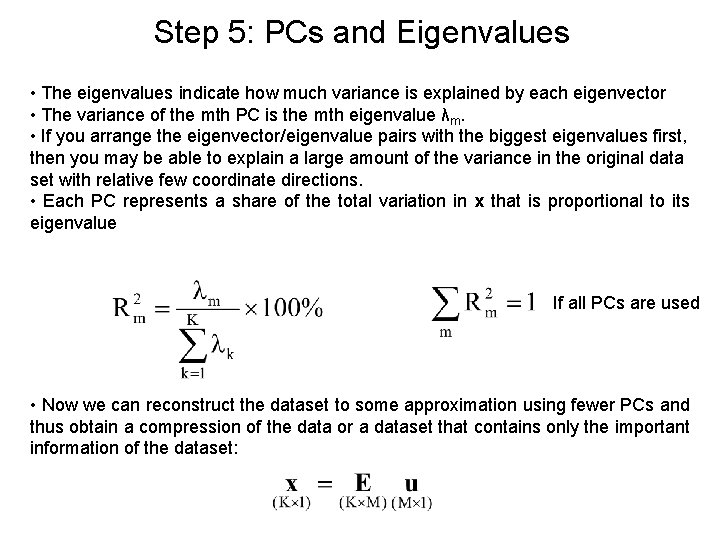
Step 5: PCs and Eigenvalues • The eigenvalues indicate how much variance is explained by each eigenvector • The variance of the mth PC is the mth eigenvalue λm. • If you arrange the eigenvector/eigenvalue pairs with the biggest eigenvalues first, then you may be able to explain a large amount of the variance in the original data set with relative few coordinate directions. • Each PC represents a share of the total variation in x that is proportional to its eigenvalue If all PCs are used • Now we can reconstruct the dataset to some approximation using fewer PCs and thus obtain a compression of the data or a dataset that contains only the important information of the dataset:

2 -D example of PCAs