Principal Component Analysis PCA Producing a new set

Principal Component Analysis PCA

Producing a new set of variables that is close to the original data – basically, trying to ID a new variable that contains most of the variability in the old data Reduce dimensionality (in this context, reduce the number of bands) Enhance contrast by maximizing the amount of information in the first three bands. Often can share PC transformed images, when you cannot do so with the original data.

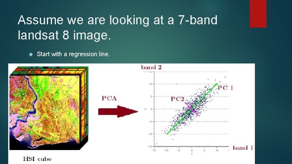
Assume we are looking at a 7 -band landsat 8 image. Start with a regression line.

I like to think of PCA as rotating axes. First PCA is the line of best fit (regression line). Every other one is at 90 degrees to the other. Easy to visualize in 2 d or 3 d space. Computers can do it in as many dimensions as you want.

When you run it You get as many principal components as you have bands. However Each PC has less and less unique information in it. As we are looking at shared variance.

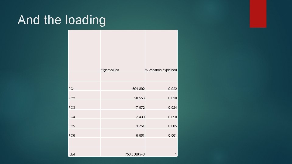
Typically PC 1 explains 60 -90% of the data PC 2 explains 10 -30% PC 3 explains 3 -15% Generally speaking, Ignore PCs that explain less than 1% of the variance. This is basically noise. 1 -3%, maybe use/keep 3% plus, this is good stuff.

Remember! There is absolutely ZERO correlation between principal components.

Generally, but it depends on your study area (use your brain) PC 1 is a general brightness component (think, sorta, a panchromatic image over the full spectrum) PC 2 is often greenness (if there’s a lot of veg) PC 3 is often wetness (if water varies across your image).

OK. Let’s run this on our Landsat 7 kimberly image and see what we get

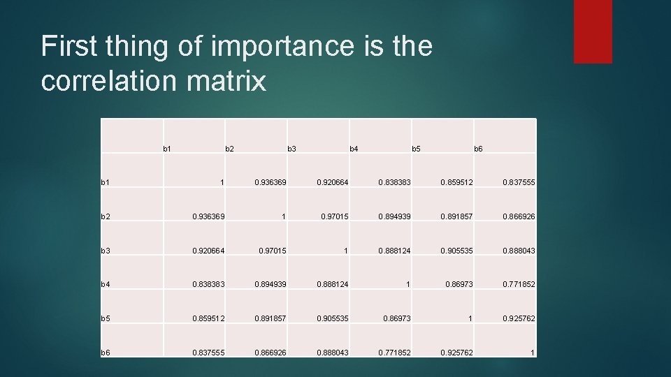
First thing of importance is the correlation matrix b 1 b 2 b 3 b 4 b 5 b 6 b 1 1 0. 936369 0. 920664 0. 838383 0. 859512 0. 837555 b 2 0. 936369 1 0. 97015 0. 894939 0. 891857 0. 866926 b 3 0. 920664 0. 97015 1 0. 888124 0. 905535 0. 888043 b 4 0. 838383 0. 894939 0. 888124 1 0. 86973 0. 771852 b 5 0. 859512 0. 891857 0. 905535 0. 86973 1 0. 925762 b 6 0. 837555 0. 866926 0. 888043 0. 771852 0. 925762 1

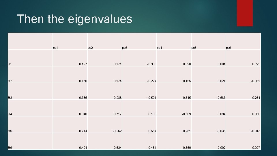
Then the eigenvalues pc 1 pc 2 pc 3 pc 4 pc 5 pc 6 B 1 0. 197 0. 171 -0. 300 0. 390 0. 801 0. 223 B 2 0. 170 0. 174 -0. 224 0. 155 0. 021 -0. 931 B 3 0. 355 0. 288 -0. 501 0. 345 -0. 583 0. 284 B 4 0. 340 0. 717 0. 186 -0. 569 0. 094 0. 058 B 5 0. 714 -0. 262 0. 584 0. 281 -0. 035 -0. 013 B 6 0. 424 -0. 524 -0. 484 -0. 550 0. 092 0. 007

And the loading Eigenvalues % variance explained PC 1 694. 892 0. 922 PC 2 28. 556 0. 038 PC 3 17. 872 0. 024 PC 4 7. 430 0. 010 PC 5 3. 751 0. 005 PC 6 0. 851 0. 001 total 753. 3509546 1

Now goto erdas and look at all the imagery