Discriminative Feature Extraction and Dimension Reduction PCA LDA

Discriminative Feature Extraction and Dimension Reduction - PCA, LDA and LSA Berlin Chen, 2005 References: 1. Introduction to Machine Learning , Chapter 6 2. Data Mining: Concepts, Models, Methods and Algorithms, Chapter 3

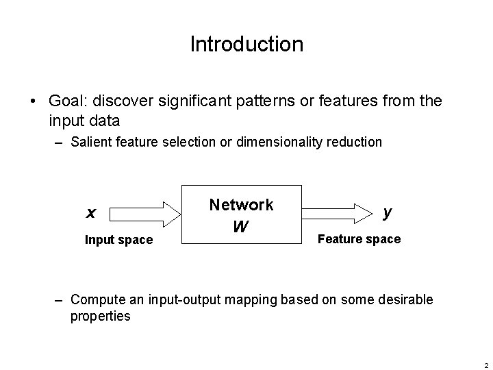
Introduction • Goal: discover significant patterns or features from the input data – Salient feature selection or dimensionality reduction x Input space Network W y Feature space – Compute an input-output mapping based on some desirable properties 2

Introduction • Principal Component Analysis (PCA) • Linear Discriminant Analysis (LDA) • Latent Semantic Analysis (LSA) • …. 3

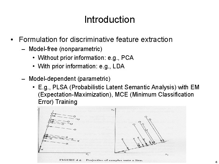
Introduction • Formulation for discriminative feature extraction – Model-free (nonparametric) • Without prior information: e. g. , PCA • With prior information: e. g. , LDA – Model-dependent (parametric) • E. g. , PLSA (Probabilistic Latent Semantic Analysis) with EM (Expectation-Maximization), MCE (Minimum Classification Error) Training 4

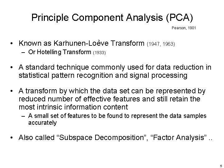
Principle Component Analysis (PCA) Pearson, 1901 • Known as Karhunen-Loẻve Transform (1947, 1963) – Or Hotelling Transform (1933) • A standard technique commonly used for data reduction in statistical pattern recognition and signal processing • A transform by which the data set can be represented by reduced number of effective features and still retain the most intrinsic information content – A small set of features to be found to represent the data samples accurately • Also called “Subspace Decomposition”, “Factor Analysis”. . 5

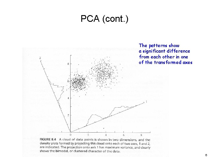
PCA (cont. ) The patterns show a significant difference from each other in one of the transformed axes 6

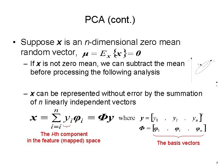
PCA (cont. ) • Suppose x is an n-dimensional zero mean random vector, – If x is not zero mean, we can subtract the mean before processing the following analysis – x can be represented without error by the summation of n linearly independent vectors The i-th component in the feature (mapped) space The basis vectors 7

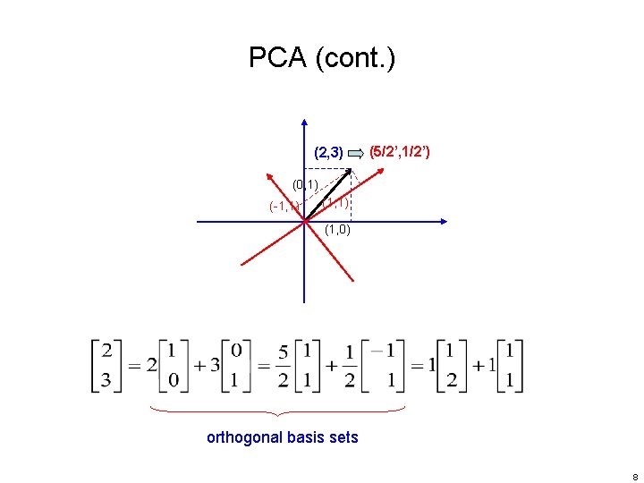
PCA (cont. ) (2, 3) (5/2’, 1/2’) (0, 1) (-1, 1) (1, 0) orthogonal basis sets 8

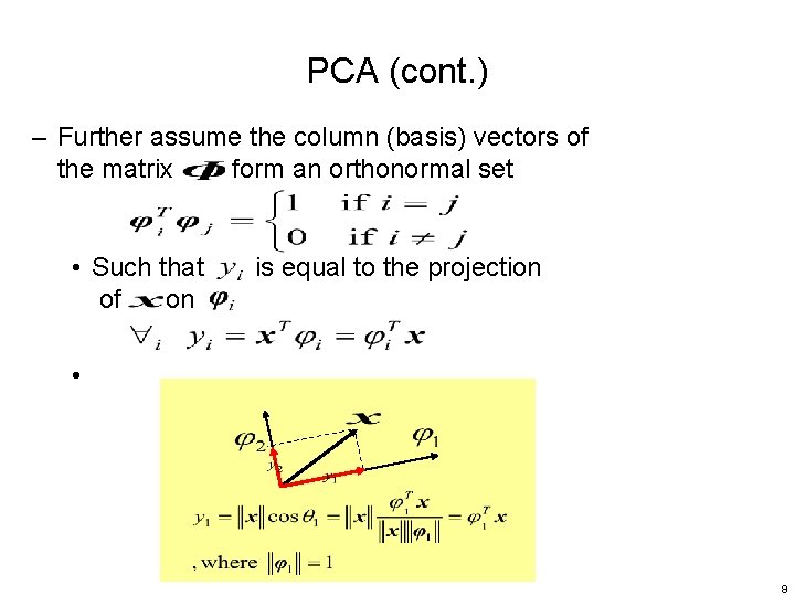
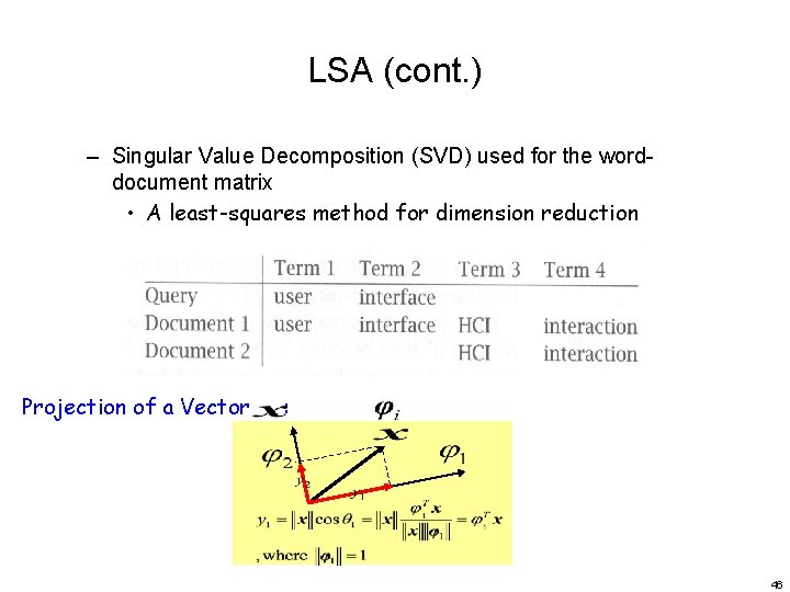
PCA (cont. ) – Further assume the column (basis) vectors of the matrix form an orthonormal set • Such that is equal to the projection of on • 9

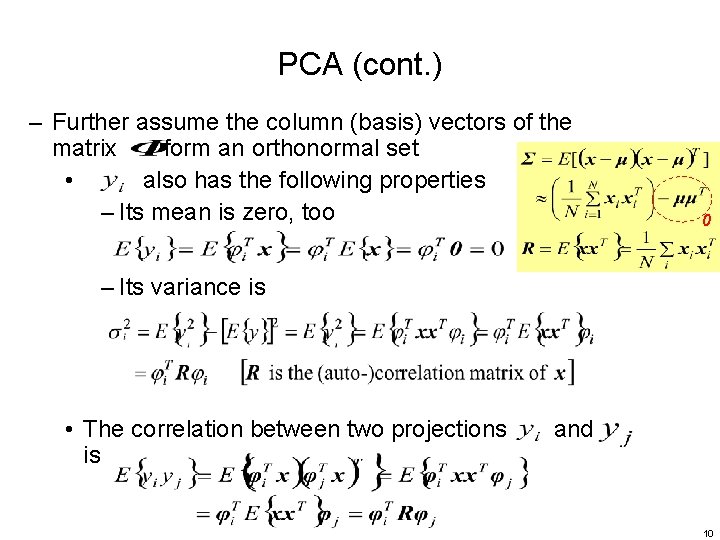
PCA (cont. ) – Further assume the column (basis) vectors of the matrix form an orthonormal set • also has the following properties – Its mean is zero, too 0 – Its variance is • The correlation between two projections and is 10

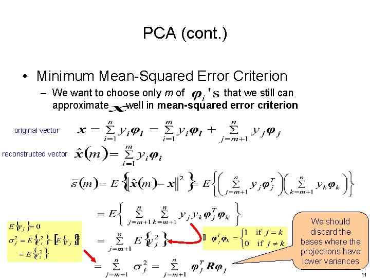
PCA (cont. ) • Minimum Mean-Squared Error Criterion – We want to choose only m of that we still can approximate well in mean-squared error criterion original vector reconstructed vector We should discard the bases where the projections have lower variances 11

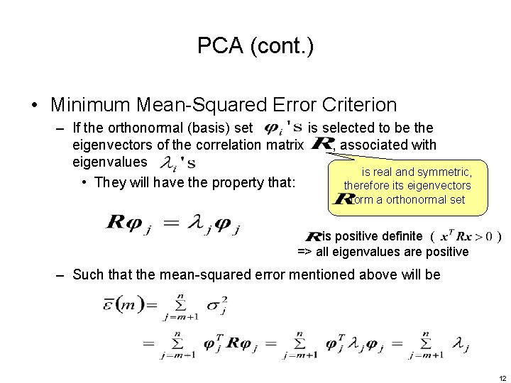
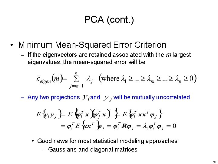
PCA (cont. ) • Minimum Mean-Squared Error Criterion – If the orthonormal (basis) set is selected to be the eigenvectors of the correlation matrix , associated with eigenvalues is real and symmetric, • They will have the property that: therefore its eigenvectors form a orthonormal set is positive definite ( ) => all eigenvalues are positive – Such that the mean-squared error mentioned above will be 12

PCA (cont. ) • Minimum Mean-Squared Error Criterion – If the eigenvectors are retained associated with the m largest eigenvalues, the mean-squared error will be – Any two projections and will be mutually uncorrelated • Good news for most statistical modeling approaches – Gaussians and diagonal matrices 13

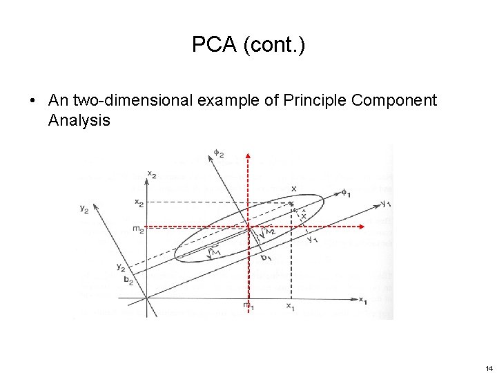
PCA (cont. ) • An two-dimensional example of Principle Component Analysis 14

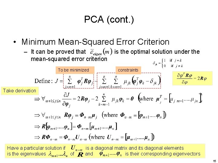
PCA (cont. ) • Minimum Mean-Squared Error Criterion – It can be proved that is the optimal solution under the mean-squared error criterion To be minimized constraints Take derivation Have a particular solution if is a diagonal matrix and its diagonal elements is the eigenvalues of and is their corresponding eigenvectors 15

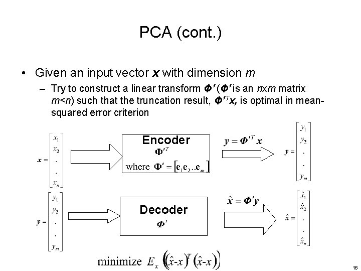
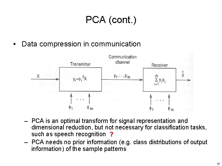
PCA (cont. ) • Given an input vector x with dimension m – Try to construct a linear transform Φ’ (Φ’ is an nxm matrix m<n) such that the truncation result, Φ’Tx, is optimal in meansquared error criterion Encoder Decoder 16

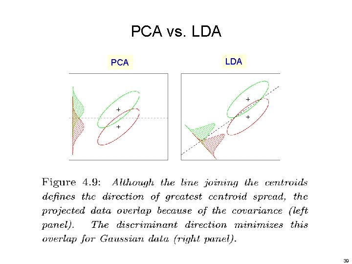
PCA (cont. ) • Data compression in communication – PCA is an optimal transform for signal representation and dimensional reduction, but not necessary for classification tasks, such as speech recognition ? – PCA needs no prior information (e. g. class distributions of output information) of the sample patterns 17

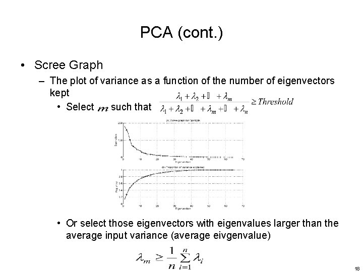
PCA (cont. ) • Scree Graph – The plot of variance as a function of the number of eigenvectors kept • Select such that • Or select those eigenvectors with eigenvalues larger than the average input variance (average eivgenvalue) 18

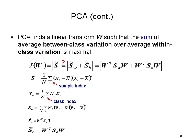
PCA (cont. ) • PCA finds a linear transform W such that the sum of average between-class variation over average withinclass variation is maximal ? sample index class index 19

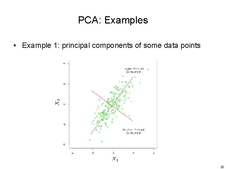
PCA: Examples • Example 1: principal components of some data points 20

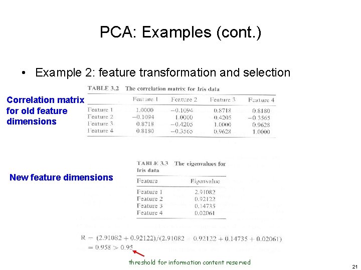
PCA: Examples (cont. ) • Example 2: feature transformation and selection Correlation matrix for old feature dimensions New feature dimensions threshold for information content reserved 21

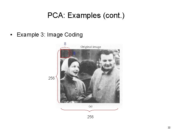
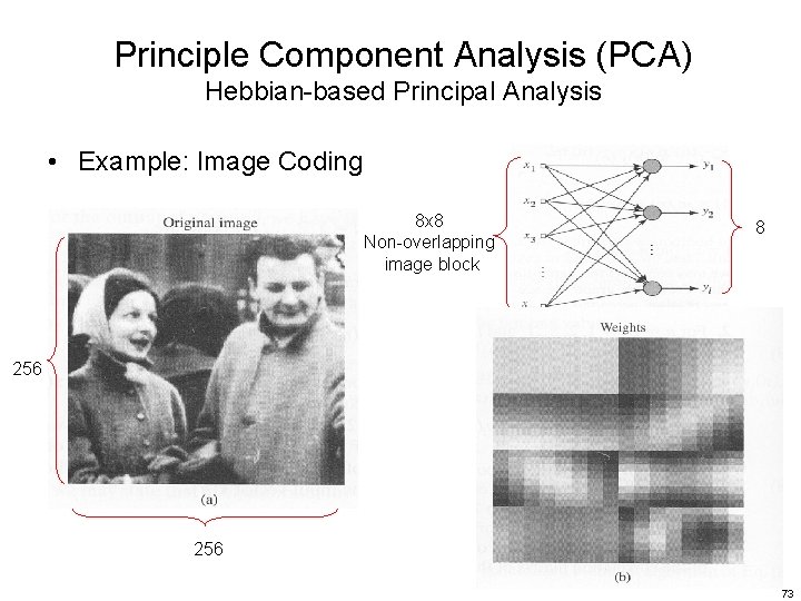
PCA: Examples (cont. ) • Example 3: Image Coding 8 8 256 22

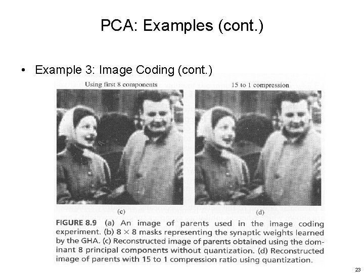
PCA: Examples (cont. ) • Example 3: Image Coding (cont. ) 23

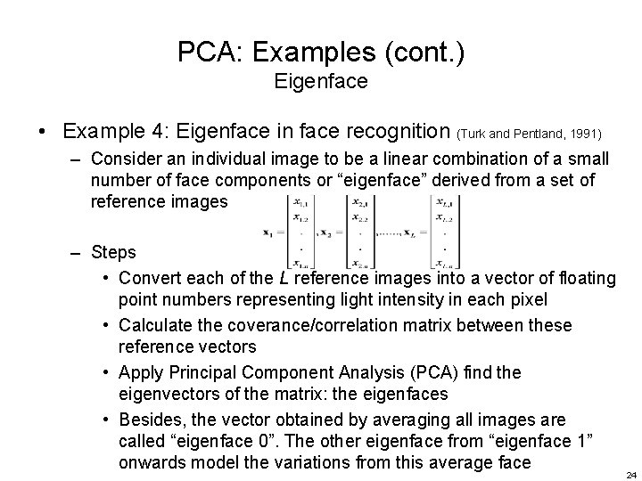
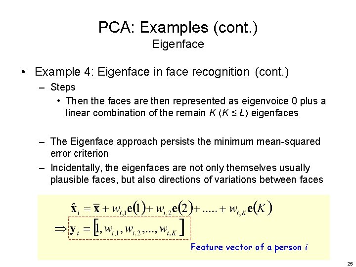
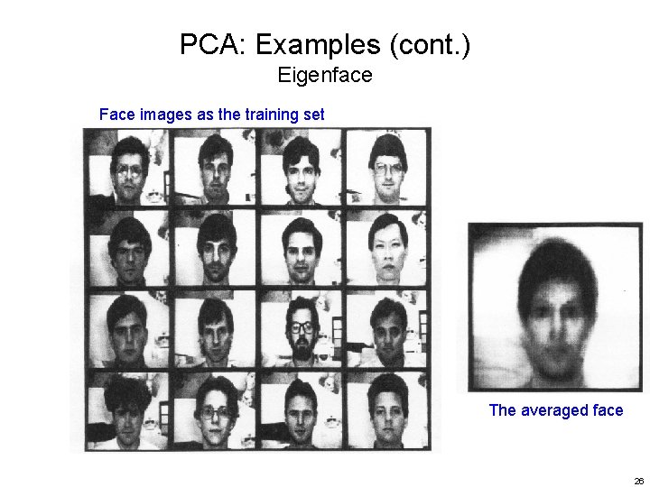
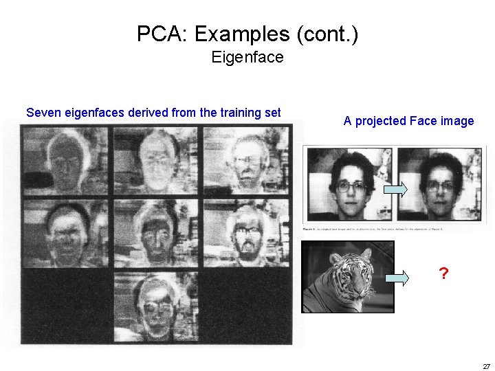
PCA: Examples (cont. ) Eigenface • Example 4: Eigenface in face recognition (Turk and Pentland, 1991) – Consider an individual image to be a linear combination of a small number of face components or “eigenface” derived from a set of reference images – Steps • Convert each of the L reference images into a vector of floating point numbers representing light intensity in each pixel • Calculate the coverance/correlation matrix between these reference vectors • Apply Principal Component Analysis (PCA) find the eigenvectors of the matrix: the eigenfaces • Besides, the vector obtained by averaging all images are called “eigenface 0”. The other eigenface from “eigenface 1” onwards model the variations from this average face 24

PCA: Examples (cont. ) Eigenface • Example 4: Eigenface in face recognition (cont. ) – Steps • Then the faces are then represented as eigenvoice 0 plus a linear combination of the remain K (K ≤ L) eigenfaces – The Eigenface approach persists the minimum mean-squared error criterion – Incidentally, the eigenfaces are not only themselves usually plausible faces, but also directions of variations between faces Feature vector of a person i 25

PCA: Examples (cont. ) Eigenface Face images as the training set The averaged face 26

PCA: Examples (cont. ) Eigenface Seven eigenfaces derived from the training set A projected Face image ? 27

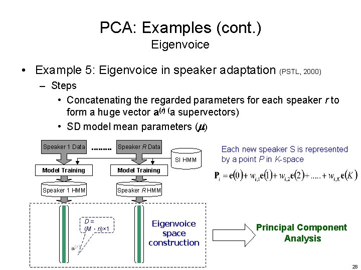
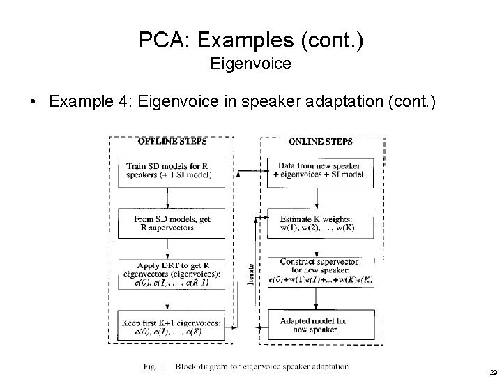
PCA: Examples (cont. ) Eigenvoice • Example 5: Eigenvoice in speaker adaptation (PSTL, 2000) – Steps • Concatenating the regarded parameters for each speaker r to form a huge vector a(r) (a supervectors) • SD model mean parameters (m) Speaker 1 Data Speaker R Data SI HMM Model Training Speaker 1 HMM Speaker R HMM D= (M．n)× 1 Eigenvoice space construction Each new speaker S is represented by a point P in K-space Principal Component Analysis 28

PCA: Examples (cont. ) Eigenvoice • Example 4: Eigenvoice in speaker adaptation (cont. ) 29

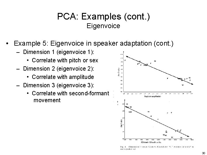
PCA: Examples (cont. ) Eigenvoice • Example 5: Eigenvoice in speaker adaptation (cont. ) – Dimension 1 (eigenvoice 1): • Correlate with pitch or sex – Dimension 2 (eigenvoice 2): • Correlate with amplitude – Dimension 3 (eigenvoice 3): • Correlate with second-formant movement 30

Linear Discriminant Analysis (LDA) • Also called – Fisher’s Linear Discriminant Analysis, Fisher-Rao Linear Discriminant Analysis • Fisher (1936): introduced it for two-classification • Rao (1965): extended it to handle multiple-classification 31

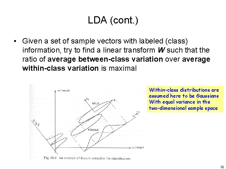
LDA (cont. ) • Given a set of sample vectors with labeled (class) information, try to find a linear transform W such that the ratio of average between-class variation over average within-class variation is maximal Within-class distributions are assumed here to be Gaussians With equal variance in the two-dimensional sample space 32

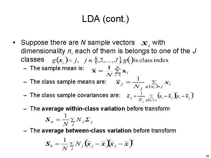
LDA (cont. ) • Suppose there are N sample vectors with dimensionality n, each of them is belongs to one of the J classes – The sample mean is: – The class sample means are: – The class sample covariances are: – The average within-class variation before transform – The average between-class variation before transform 33

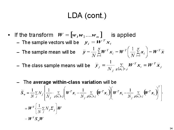
LDA (cont. ) • If the transform is applied – The sample vectors will be – The sample mean will be – The class sample means will be – The average within-class variation will be 34

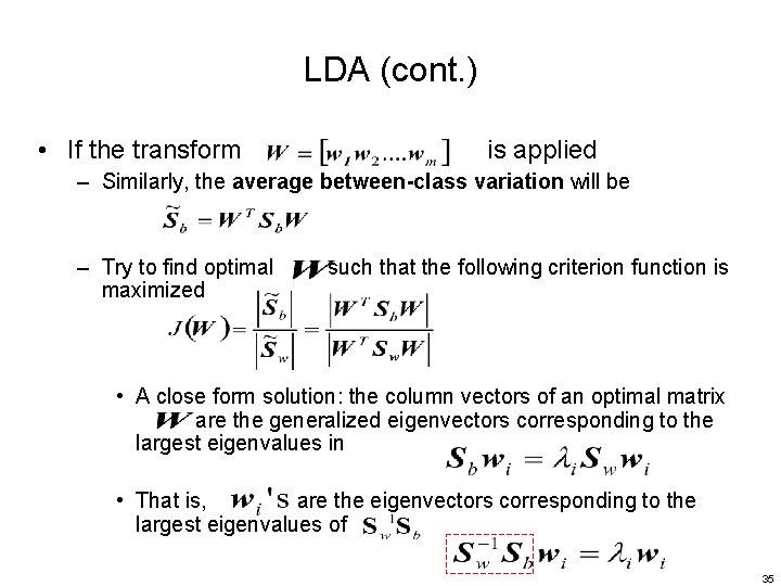
LDA (cont. ) • If the transform is applied – Similarly, the average between-class variation will be – Try to find optimal such that the following criterion function is maximized • A close form solution: the column vectors of an optimal matrix are the generalized eigenvectors corresponding to the largest eigenvalues in • That is, are the eigenvectors corresponding to the largest eigenvalues of 35

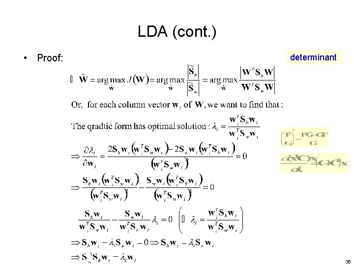
LDA (cont. ) • Proof: determinant 36

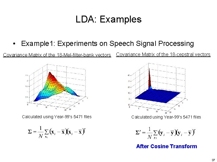
LDA: Examples • Example 1: Experiments on Speech Signal Processing Covariance Matrix of the 18 -Mel-filter-bank vectors Calculated using Year-99’s 5471 files Covariance Matrix of the 18 -cepstral vectors Calculated using Year-99’s 5471 files After Cosine Transform 37

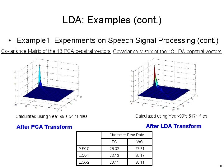
LDA: Examples (cont. ) • Example 1: Experiments on Speech Signal Processing (cont. ) Covariance Matrix of the 18 -PCA-cepstral vectors Covariance Matrix of the 18 -LDA-cepstral vectors Calculated using Year-99’s 5471 files After LDA Transform After PCA Transform Character Error Rate TC WG MFCC 26. 32 22. 71 LDA-1 23. 12 20. 17 LDA-2 23. 11 20. 11 38

PCA vs. LDA PCA LDA 39

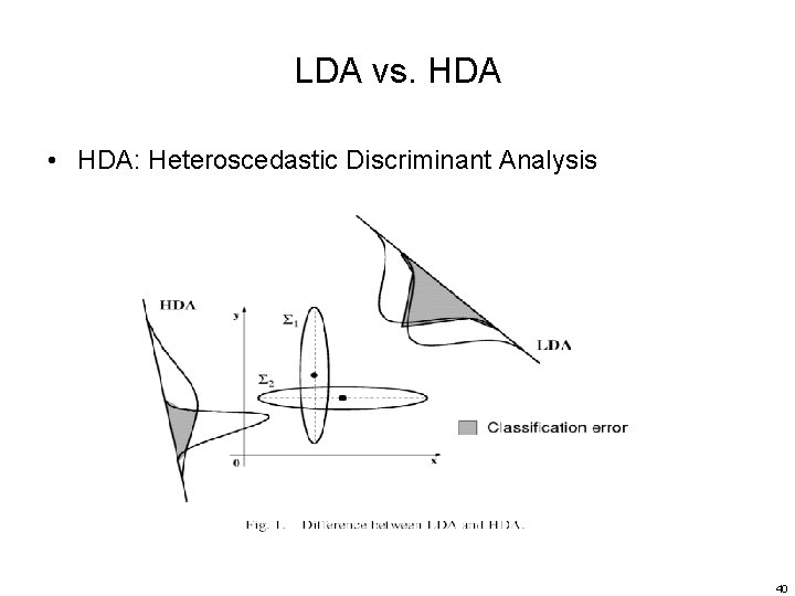
LDA vs. HDA • HDA: Heteroscedastic Discriminant Analysis 40

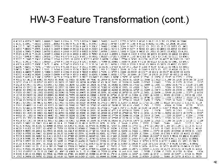
HW-3 Feature Transformation • Given two data sets (Male. Data, Female. Data) in which each row is a sample with 39 features, please perform the following operations: 1. Merge these two data sets and find/plot the covariance matrix for the merged data set. 2. Apply PCA and LDA transformations to the merged data set, respectively. Also, find/plot the covariance matrices for transformations, respectively. Describe the phenomena that you have observed. 3. Use the first two principal components of PCA as well as the first two eigenvectors of LDA to represent the merged data set. Selectively plot portions of samples from Male. Data and Female. Data, respectively. Describe the phenomena that you have observed. 41

HW-3 Feature Transformation (cont. ) 42

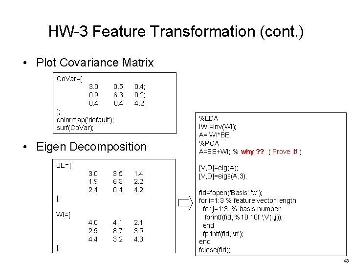
HW-3 Feature Transformation (cont. ) • Plot Covariance Matrix Co. Var=[ 3. 0 0. 5 0. 4; 0. 9 6. 3 0. 2; 0. 4 4. 2; ]; colormap('default'); surf(Co. Var); • Eigen Decomposition BE=[ 3. 0 3. 5 1. 4; 1. 9 6. 3 2. 2; 2. 4 0. 4 4. 2; ]; WI=[ 4. 0 4. 1 2. 1; 2. 9 8. 7 3. 5; 4. 4 3. 2 4. 3; ]; %LDA IWI=inv(WI); A=IWI*BE; %PCA A=BE+WI; % why ? ? ( Prove it! ) [V, D]=eig(A); [V, D]=eigs(A, 3); fid=fopen('Basis', 'w'); for i=1: 3 % feature vector length for j=1: 3 % basis number fprintf(fid, '%10. 10 f ', V(i, j)); end fprintf(fid, 'n'); end fclose(fid); 43

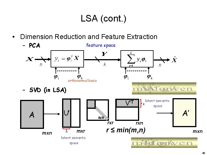
Latent Semantic Analysis (LSA) • Also called Latent Semantic Indexing (LSI), Latent Semantic Mapping (LSM) • A technique originally proposed for Information Retrieval (IR), which projects queries and docs into a space with “latent” semantic dimensions – Co-occurring terms are projected onto the same dimensions – In the latent semantic space (with fewer dimensions), a query and doc can have high cosine similarity even if they do not share any terms – Dimensions of the reduced space correspond to the axes of greatest variation • Closely related to Principal Component Analysis (PCA) 44

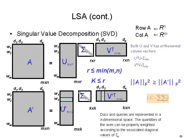
LSA (cont. ) • Dimension Reduction and Feature Extraction – PCA feature space k n n orthonormal basis – SVD (in LSA) Σ’ U’ A V’T k latent semantic space kxk rxr mxn k mxr A’ rxn r ≤ min(m, n) mxn latent semantic space 45

LSA (cont. ) – Singular Value Decomposition (SVD) used for the worddocument matrix • A least-squares method for dimension reduction Projection of a Vector : 46

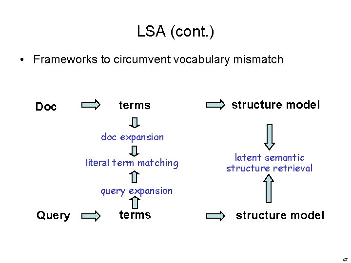
LSA (cont. ) • Frameworks to circumvent vocabulary mismatch Doc terms structure model doc expansion literal term matching latent semantic structure retrieval query expansion Query terms structure model 47

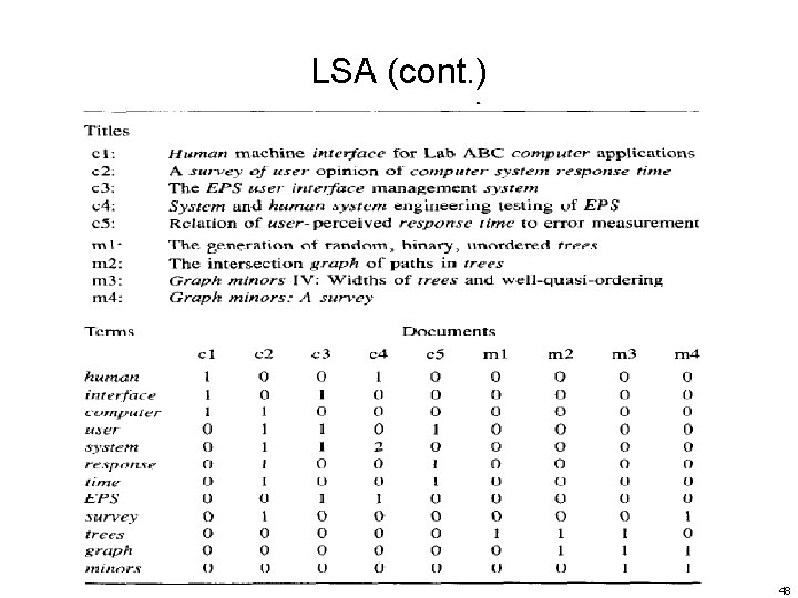
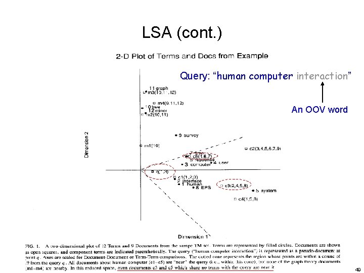
LSA (cont. ) 48

LSA (cont. ) Query: “human computer interaction” An OOV word 49

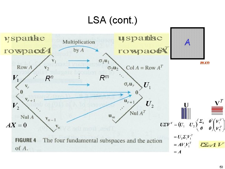
LSA (cont. ) • Singular Value Decomposition (SVD) d 1 d 2 dn w 1 w 2 A Umxr = d 1 d 2 A’ U’mxk dn ||A||F 2 ≥ ||A’|| F 2 V’Tkxm kxk wm UTU=Ir. Xr VTV=Ir. Xr K≤r Σk w 1 w 2 = mxn rxn d 1 d 2 w 1 w 2 rxm r ≤ min(m, n) mxr mxn dn Both U and V has orthonormal column vectors rxr wm wm wm Σr VT dn Row A Rn Col A Rm kxn Docs and queries are represented in a k-dimensional space. The quantities of the axes can be properly weighted according to the associated diagonal values of Σk 50

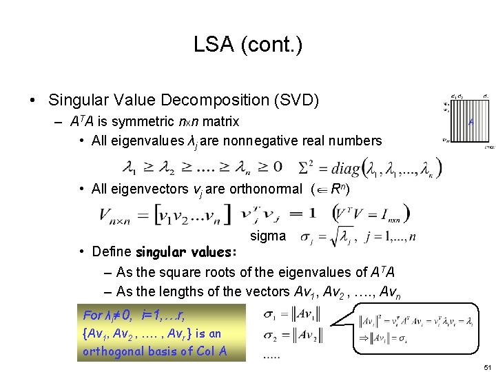
LSA (cont. ) • Singular Value Decomposition (SVD) – ATA is symmetric nxn matrix • All eigenvalues λj are nonnegative real numbers • All eigenvectors vj are orthonormal ( Rn) sigma • Define singular values: – As the square roots of the eigenvalues of ATA – As the lengths of the vectors Av 1, Av 2 , …. , Avn For λi≠ 0, i=1, …r, {Av 1, Av 2 , …. , Avr } is an orthogonal basis of Col A 51

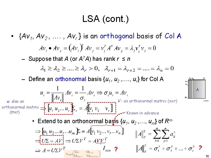
LSA (cont. ) • {Av 1, Av 2 , …. , Avr } is an orthogonal basis of Col A – Suppose that A (or ATA) has rank r ≤ n – Define an orthonormal basis {u 1, u 2 , …. , ur} for Col A u: also an orthonormal matrix (mxr) V : an orthonormal matrix (nxr) Known in advance • Extend to an orthonormal basis {u 1, u 2 , …, um} of Rm ? ? 52

LSA (cont. ) A mxn Rn Rm 53

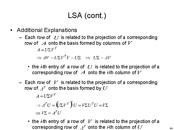
LSA (cont. ) • Additional Explanations – Each row of is related to the projection of a corresponding row of onto the basis formed by columns of • the i-th entry of a row of is related to the projection of a corresponding row of onto the i-th column of – Each row of is related to the projection of a corresponding row of onto the basis formed by • the i-th entry of a row of is related to the projection of a corresponding row of onto the i-th column of 54

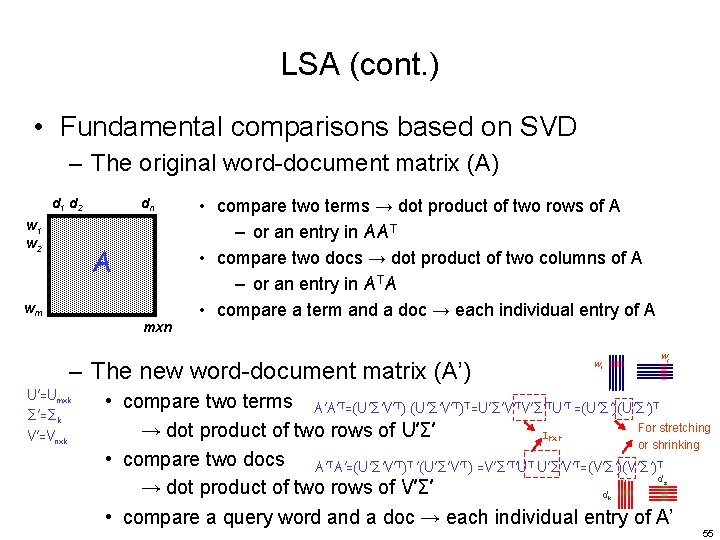
LSA (cont. ) • Fundamental comparisons based on SVD – The original word-document matrix (A) d 1 d 2 w 1 w 2 dn A wm mxn • compare two terms → dot product of two rows of A – or an entry in AAT • compare two docs → dot product of two columns of A – or an entry in ATA • compare a term and a doc → each individual entry of A – The new word-document matrix (A’) U’=Umxk Σ’=Σk V’=Vnxk wj wi • compare two terms A’A’T=(U’Σ’V’T)T=U’Σ’V’TV’Σ’TU’T =(U’Σ’)T For stretching → dot product of two rows of U’Σ’ Irxr or shrinking • compare two docs A’TA’=(U’Σ’V’T)T ’(U’Σ’V’T) =V’Σ’T’UT U’Σ’V’T=(V’Σ’)T d → dot product of two rows of V’Σ’ d • compare a query word and a doc → each individual entry of A’ s k 55

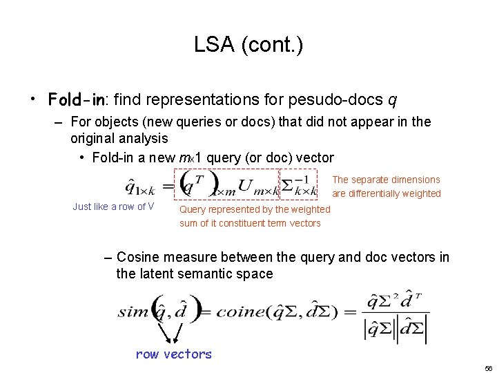
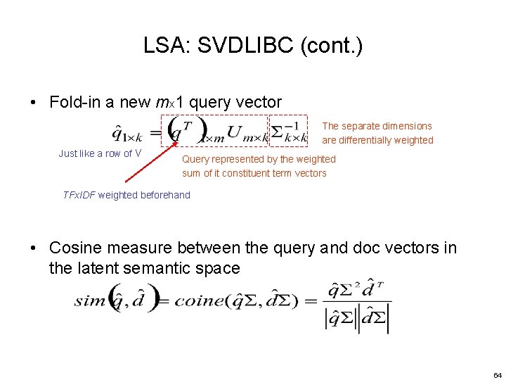
LSA (cont. ) • Fold-in: find representations for pesudo-docs q – For objects (new queries or docs) that did not appear in the original analysis • Fold-in a new mx 1 query (or doc) vector The separate dimensions are differentially weighted Just like a row of V Query represented by the weighted sum of it constituent term vectors – Cosine measure between the query and doc vectors in the latent semantic space row vectors 56

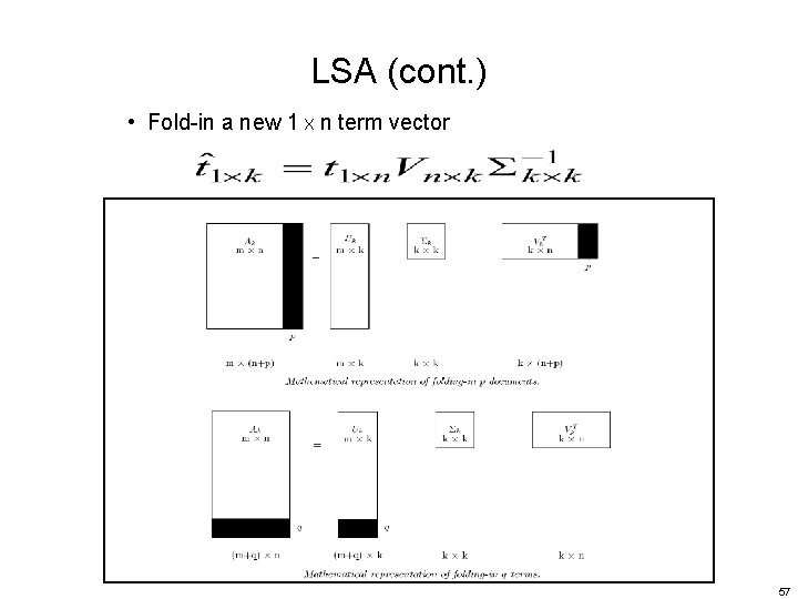
LSA (cont. ) • Fold-in a new 1 X n term vector 57

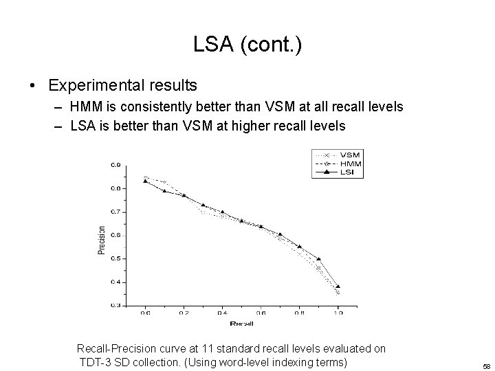
LSA (cont. ) • Experimental results – HMM is consistently better than VSM at all recall levels – LSA is better than VSM at higher recall levels Recall-Precision curve at 11 standard recall levels evaluated on TDT-3 SD collection. (Using word-level indexing terms) 58

LSA (cont. ) • Advantages – A clean formal framework and a clearly defined optimization criterion (least-squares) • Conceptual simplicity and clarity – Handle synonymy problems (“heterogeneous vocabulary”) – Good results for high-recall search • Take term co-occurrence into account • Disadvantages – High computational complexity – LSA offers only a partial solution to polysemy • E. g. bank, bass, … 59

LSA: SVDLIBC • Doug Rohde's SVD C Library version 1. 3 is based on the SVDPACKC library • Download it at http: //tedlab. mit. edu/~dr/ 60

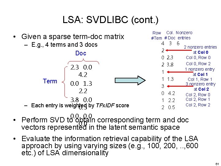
LSA: SVDLIBC (cont. ) • Given a sparse term-doc matrix – E. g. , 4 terms and 3 docs Doc • Row Col. Nonzero #Tem # Doc entries 4 3 6 2 nonzero entries 2 at Col 0, Row 0 0 2. 3 Col 0, Row 2 2 3. 8 1 nonzero entry 1 at Col 1 1 1. 3 Col 1, Row 1 3 nonzero entry 3 at Col 2 0 4. 2 Col 2, Row 0 Col 2, Row 1 1 2. 2 Col 2, Row 2 2 0. 5 2. 3 0. 0 4. 2 Term 0. 0 1. 3 2. 2 3. 8 0. 0 – Each entry is weighted by TFx. IDF score 0. 5 0. 0 Perform SVD to obtain corresponding term and doc 0. 0 vectors represented in the latent semantic space • Evaluate the information retrieval capability of the LSA approach by using varying sizes (e. g. , 100, 200, . . , 600 etc. ) of LSA dimensionality 61

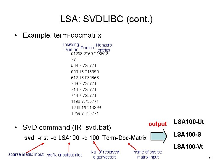
LSA: SVDLIBC (cont. ) • Example: term-docmatrix Indexing Nonzero Doc no. Term no. entries 51253 2265 218852 77 508 7. 725771 596 16. 213399 612 13. 080868 709 7. 725771 713 7. 725771 744 7. 725771 1190 7. 725771 1200 16. 213399 1259 7. 725771 …… • SVD command (IR_svd. bat) svd -r st -o LSA 100 -d 100 Term-Doc-Matrix sparse matrix input prefix of output files No. of reserved eigenvectors output name of sparse matrix input LSA 100 -Ut LSA 100 -S LSA 100 -Vt 62

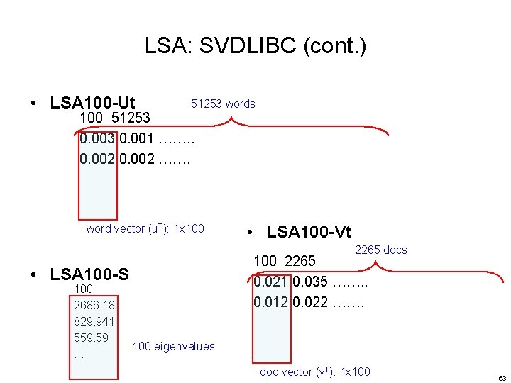
LSA: SVDLIBC (cont. ) • LSA 100 -Ut 51253 words 100 51253 0. 001 ……. . 0. 002 ……. word vector (u. T): 1 x 100 • LSA 100 -Vt 2265 docs 100 2265 0. 021 0. 035 ……. . 0. 012 0. 022 ……. • LSA 100 -S 100 2686. 18 829. 941 559. 59 …. 100 eigenvalues doc vector (v. T): 1 x 100 63

LSA: SVDLIBC (cont. ) • Fold-in a new mx 1 query vector The separate dimensions are differentially weighted Just like a row of V Query represented by the weighted sum of it constituent term vectors TFx. IDF weighted beforehand • Cosine measure between the query and doc vectors in the latent semantic space 64

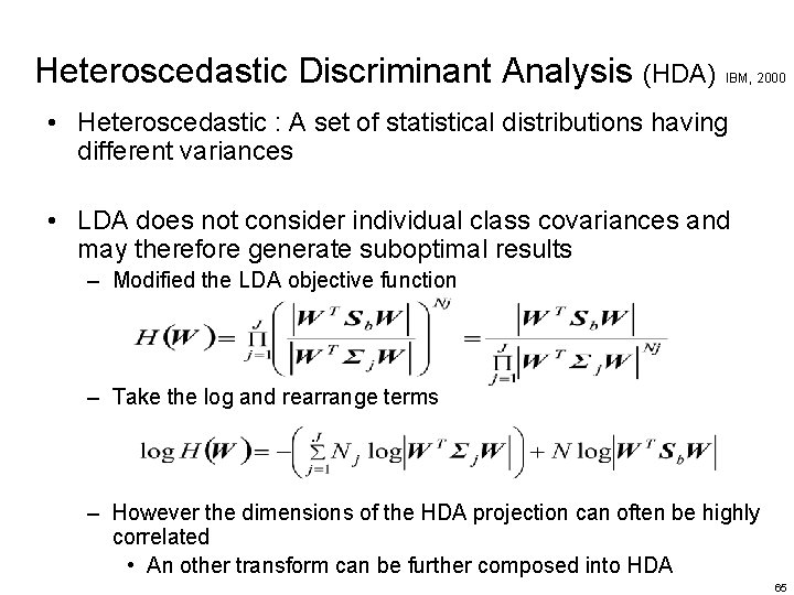
Heteroscedastic Discriminant Analysis (HDA) IBM, 2000 • Heteroscedastic : A set of statistical distributions having different variances • LDA does not consider individual class covariances and may therefore generate suboptimal results – Modified the LDA objective function – Take the log and rearrange terms – However the dimensions of the HDA projection can often be highly correlated • An other transform can be further composed into HDA 65

66

67

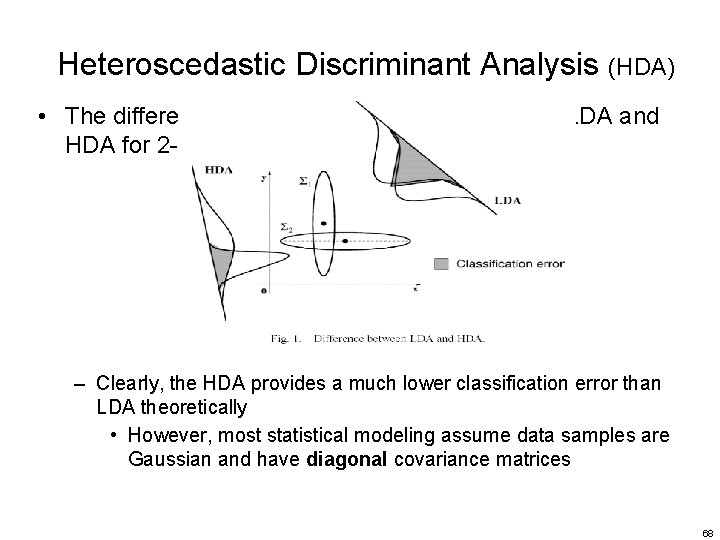
Heteroscedastic Discriminant Analysis (HDA) • The difference in the projections obtained from LDA and HDA for 2 -class case – Clearly, the HDA provides a much lower classification error than LDA theoretically • However, most statistical modeling assume data samples are Gaussian and have diagonal covariance matrices 68

69

70

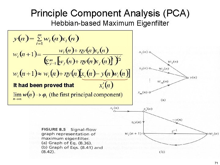
Principle Component Analysis (PCA) Hebbian-based Maximum Eigenfilter It had been proved that 71

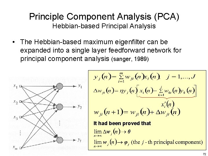
Principle Component Analysis (PCA) Hebbian-based Principal Analysis • The Hebbian-based maximum eigenfilter can be expanded into a single layer feedforward network for principal component analysis (sanger, 1989) It had been proved that 72

Principle Component Analysis (PCA) Hebbian-based Principal Analysis • Example: Image Coding 8 x 8 Non-overlapping image block 8 256 73

74

Principle Component Analysis (PCA) Adaptive Principal Components Extraction • Both feedward and lateral connections are used 75

76

Known Weakness of PCA 77