Mathematical Modeling Prof Ing Michele MICCIO Dept of

Mathematical Modeling Prof. Ing. Michele MICCIO Dept. of Industrial Engineering (Università di Salerno) Prodal Scarl (Fisciano) Rev. 7. 01 of December 10, 2014

TYPES OF MODELS Models are used not only in the natural sciences (such as physics, biology, life sciences, earth science, meteorology) and engineeringarchitecture disciplines, but also in the social sciences (such as economics, psychology, sociology and political science). Here is a list: · Physical Models Analogic Models Provisional Theories (e. g. , molecular and atomic models) Maps and Drawings (e. g. , PI&D, geographycal maps, etc. ) Mathematical and symbolic models § 1. 4 in Himmelblau D. M. e Bischoff K. B. , “Process Analysis and Simulation”, Wiley & Sons Inc. , 1967 2

Why modeling? Some answers … Models are usually more accessible to study than the actual system modeled. • Changes in the structure of a model are easier to implement, and changes in the behavior of a model are easier to isolate, understand, and communicate to others. • A model can be used to achieve insight when direct observation/experimentation with the actual system is too dangerous, disruptive, or demanding. • A model can be used to answer questions about a system that has not yet been observed or built, or even one that cannot be observed or built with present technologies. 3

MATHEMATICAL MODELING A mathematical model is a description of a system using mathematical concepts and language. The process of developing a mathematical model is termed mathematical modeling. Mathematical models are used not only in the NATURAL SCIENCES (such as physics, biology, earth science, meteorology) and ENGINEERING DISCIPLINES (e. g. computer science, artificial intelligence), but also in the SOCIAL SCIENCES (such as economics, psychology, sociology and political science); physicists, engineers, statisticians, operations research analysts and economists use mathematical models most extensively. A model may help to explain a system and to study the effects of different components, and to make predictions about behavior. 4

MATHEMATICAL MODELING General statements A mathematical model usually describes a system by a set of variables and a set of equations that establish relationships between the variables. Relationships can be described by operators, such as algebraic operators, functions, differential operators, etc. Anonymous A mathematical model is a representation, in mathematical terms, of certain aspects of a non-mathematical system Aris, 1999 A model may be prescriptive or illustrative, but, above all, it must be useful ! 5 Wilson, 1991

Why Math Modeling ? • Is it: Ø to design a controller? Ø to analyze the performance of the process? Ø to understand the process/system better? Ø to simplify the complexity of a system? 6 Introduction to Process Control Romagnoli & Palazoglu

Mathematical model development strategy • The development of a model and its structure are intimately related to the goals of modeling. • In other words, the complexity of a model should be commensurate with the ultimate application in which it will be used. • In model development, always start by trying the simplest model and then only add complexity to the extent needed Keep things as simple as possible, but not simpler A. Einstein Introduction to Process Control Romagnoli & Palazoglu 7

Mathematical model development: Complexity vs. Simplicity Ø Ratio of costs to benefits Introduction to Process Control Romagnoli & Palazoglu 8

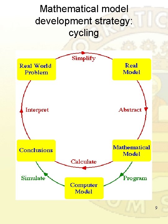
Mathematical model development strategy: cycling 9

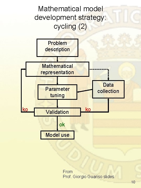
Mathematical model development strategy: cycling (2) Problem description Mathematical representation Data collection Parameter tuning ko Validation ko ok Model use From Prof. Giorgio Guariso slides 10

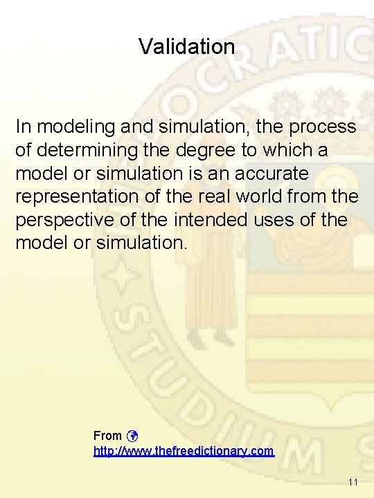
Validation In modeling and simulation, the process of determining the degree to which a model or simulation is an accurate representation of the real world from the perspective of the intended uses of the model or simulation. From http: //www. thefreedictionary. com 11

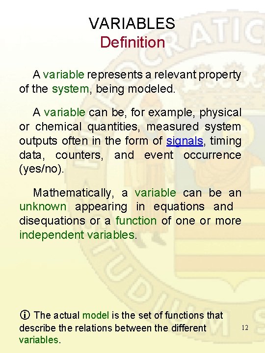
VARIABLES Definition A variable represents a relevant property of the system, being modeled. A variable can be, for example, physical or chemical quantities, measured system outputs often in the form of signals, timing data, counters, and event occurrence (yes/no). Mathematically, a variable can be an unknown appearing in equations and disequations or a function of one or more independent variables. The actual model is the set of functions that describe the relations between the different variables. 12

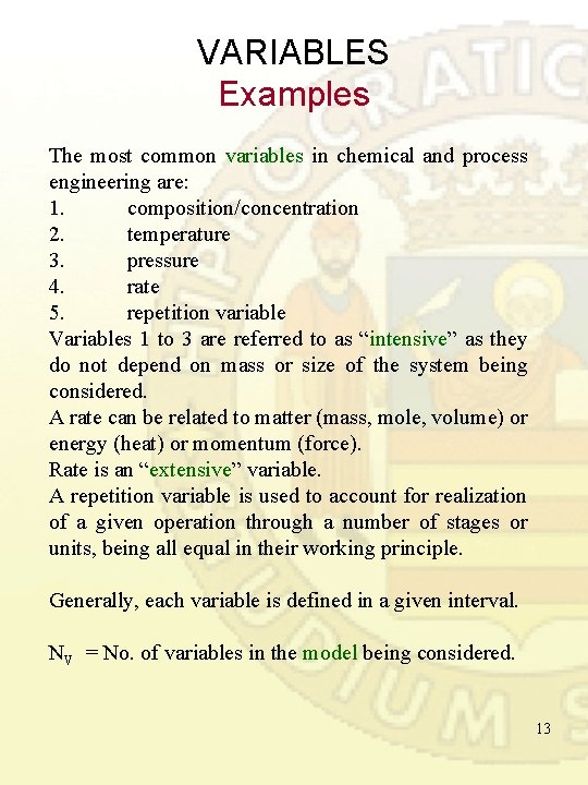
VARIABLES Examples The most common variables in chemical and process engineering are: 1. composition/concentration 2. temperature 3. pressure 4. rate 5. repetition variable Variables 1 to 3 are referred to as “intensive” as they do not depend on mass or size of the system being considered. A rate can be related to matter (mass, mole, volume) or energy (heat) or momentum (force). Rate is an “extensive” variable. A repetition variable is used to account for realization of a given operation through a number of stages or units, being all equal in their working principle. Generally, each variable is defined in a given interval. NV = No. of variables in the model being considered. 13

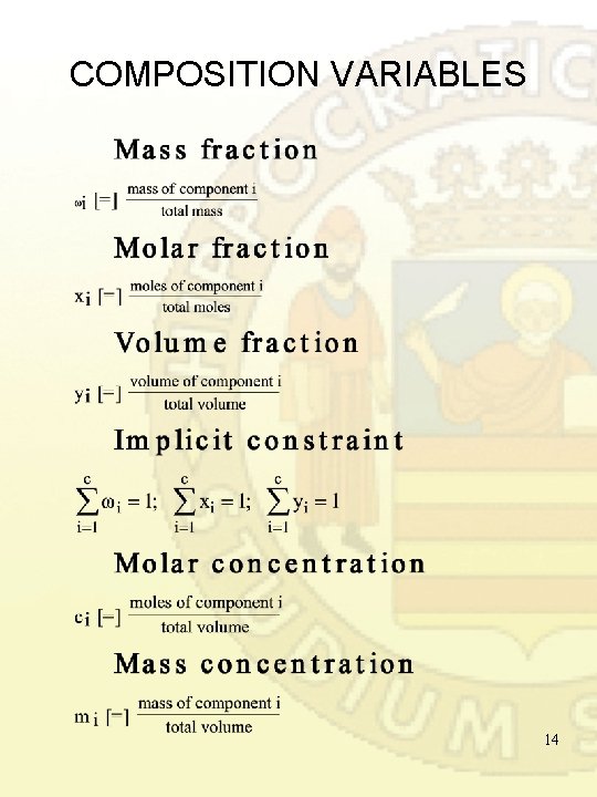
COMPOSITION VARIABLES 14

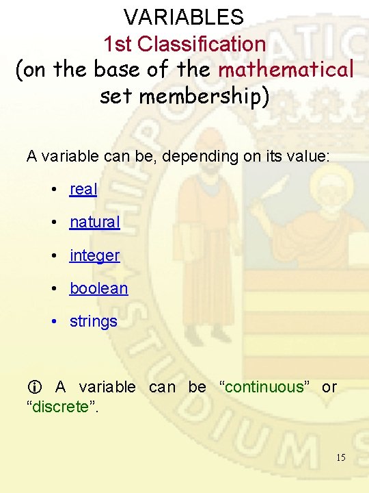
VARIABLES 1 st Classification (on the base of the mathematical set membership) A variable can be, depending on its value: • real • natural • integer • boolean • strings A variable can be “continuous” or “discrete”. 15

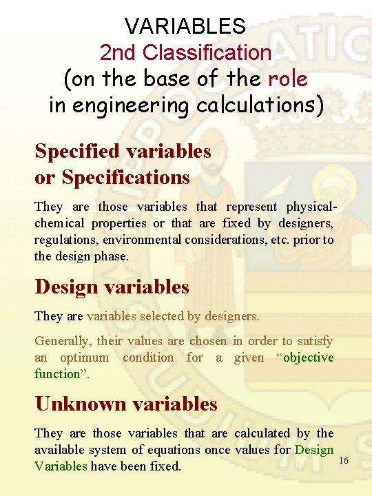
VARIABLES 2 nd Classification (on the base of the role in engineering calculations) Specified variables or Specifications They are those variables that represent physicalchemical properties or that are fixed by designers, regulations, environmental considerations, etc. prior to the design phase. Design variables They are variables selected by designers. Generally, their values are chosen in order to satisfy an optimum condition for a given “objective function”. Unknown variables They are those variables that are calculated by the available system of equations once values for Design 16 Variables have been fixed.

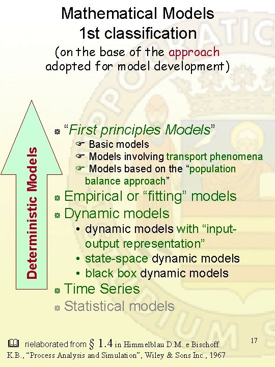
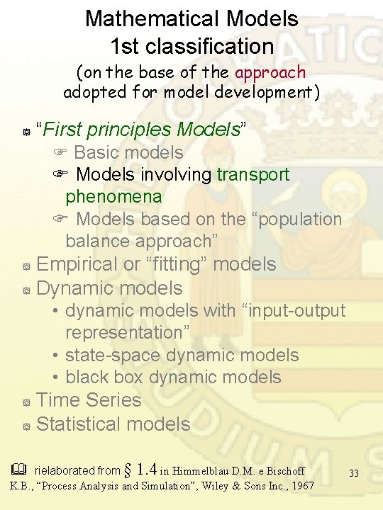
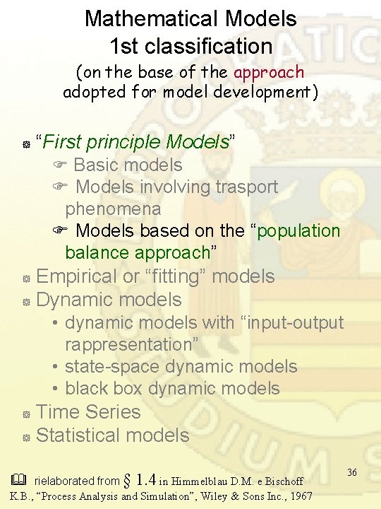
Mathematical Models 1 st classification (on the base of the approach adopted for model development) Deterministic Models ] “First principles Models” Basic models Models involving transport phenomena Models based on the “population balance approach” Empirical or “fitting” models ] Dynamic models ] • dynamic models with “inputoutput representation” • state-space dynamic models • black box dynamic models Time Series ] Statistical models ] rielaborated from § 1. 4 in Himmelblau D. M. e Bischoff K. B. , “Process Analysis and Simulation”, Wiley & Sons Inc. , 1967 17

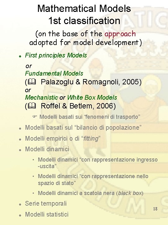
Mathematical Models 1 st classification (on the base of the approach adopted for model development) ] First principles Models or Fundamental Models ( Palazoglu & Romagnoli, 2005) or Mechanistic or White Box Models ( Roffel & Betlem, 2006) Modelli basati sui “fenomeni di trasporto” ] Modelli basati sul “bilancio di popolazione” ] Modelli empirici o di “fitting” ] Modelli dinamici • Modelli dinamici “con rappresentazione ingresso -uscita” • Modelli dinamici “con rappresentazione nello spazio di stato” • Modelli dinamici a scatola nera (black box) ] Serie temporali ] Modelli statistici 18

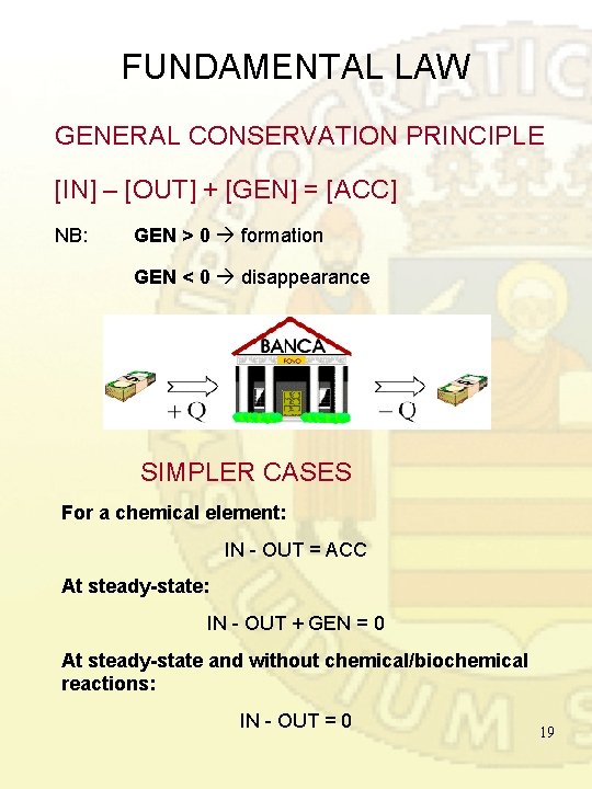
FUNDAMENTAL LAW GENERAL CONSERVATION PRINCIPLE [IN] – [OUT] + [GEN] = [ACC] NB: GEN > 0 formation GEN < 0 disappearance SIMPLER CASES For a chemical element: IN - OUT = ACC At steady-state: IN - OUT + GEN = 0 At steady-state and without chemical/biochemical reactions: IN - OUT = 0 19

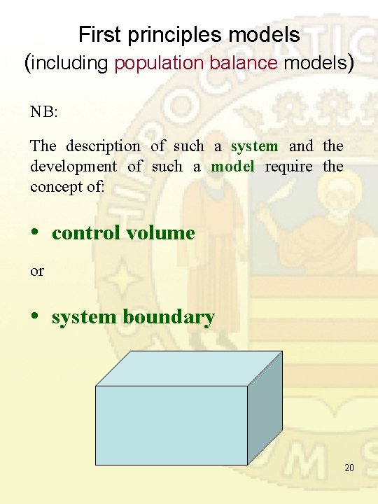
First principles models (including population balance models) NB: The description of such a system and the development of such a model require the concept of: • control volume or • system boundary 20

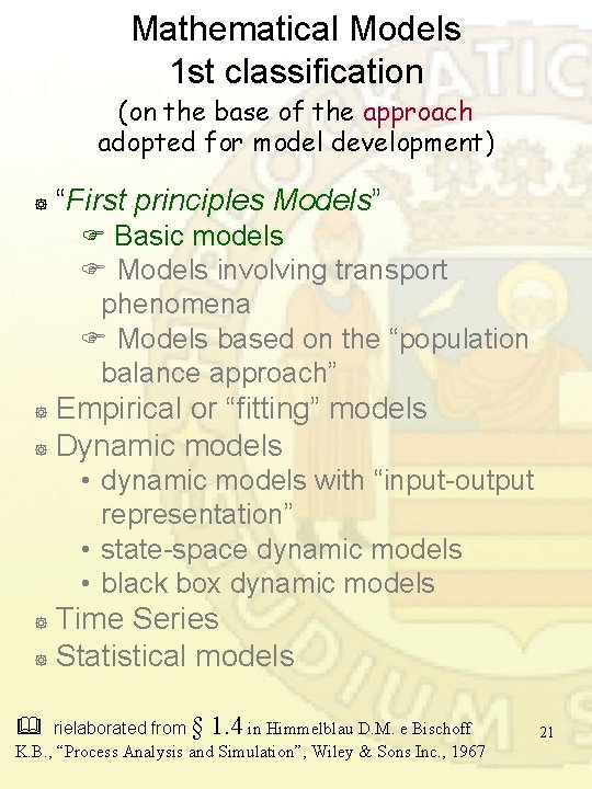
Mathematical Models 1 st classification (on the base of the approach adopted for model development) ] “First principles Models” Basic models Models involving transport phenomena Models based on the “population balance approach” Empirical or “fitting” models ] Dynamic models ] • dynamic models with “input-output representation” • state-space dynamic models • black box dynamic models Time Series ] Statistical models ] rielaborated from § 1. 4 in Himmelblau D. M. e Bischoff K. B. , “Process Analysis and Simulation”, Wiley & Sons Inc. , 1967 21

First principles mathematical models. Malthusian Growth Model An Early and Very Famous Population Model In 1798 the Englishman Thomas R. Malthus posited a mathematical model of population growth. He model, though simple, has become a basis for most future modeling of biological populations. His essay, "An Essay on the Principle of Population, " contains an excellent discussion of the caveats of mathematical modeling and should be required reading for all serious students of the discipline. Malthus's observation was that, unchecked by environmental or social constraints, it appeared that human populations doubled every twenty-five years, regardless of the initial population size. Said another way, he posited that populations increased by a fixed proportion over a given period of time and that, absent constraints, this proportion was not affected by the size of the population. By way of example, according to Malthus, if a population of 100 individuals increased to a population 135 individuals over the course of, say, five years, then a population of 1000 individuals would increase to 1350 individuals over the same period of time. Malthus's model is an example of a model with one variable and one parameter. A variable is the quantity we are interested in observing. They usually change over time. Parameters are quantities which are known to the modeler before the model is constructed. Often they are constants, although it is possible for a parameter to change over time. In the Malthusian model the variable is the population and the parameter is the population growth rate. 22

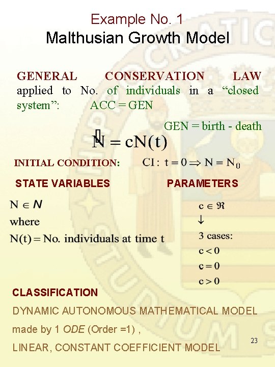
Example No. 1 Malthusian Growth Model GENERAL CONSERVATION LAW applied to No. of individuals in a “closed system”: ACC = GEN = birth - death INITIAL CONDITION: STATE VARIABLES PARAMETERS CLASSIFICATION DYNAMIC AUTONOMOUS MATHEMATICAL MODEL made by 1 ODE (Order =1) , LINEAR, CONSTANT COEFFICIENT MODEL 23

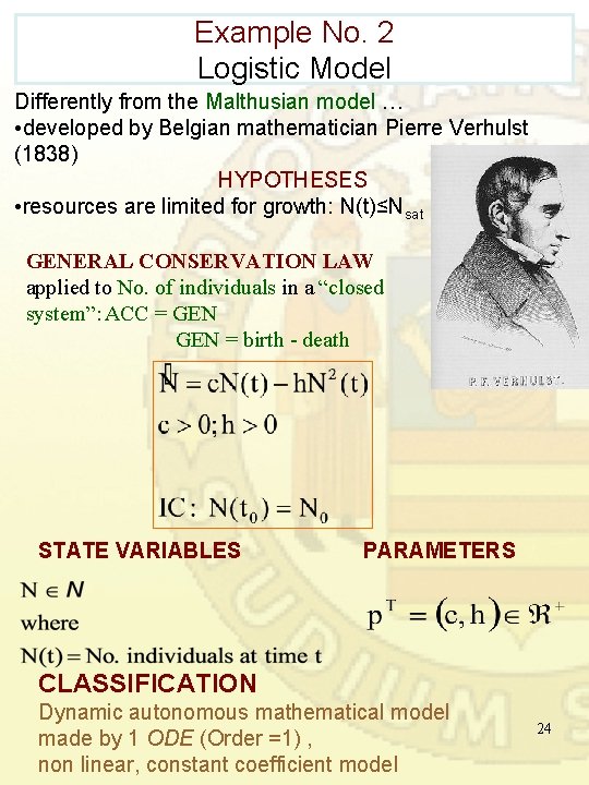
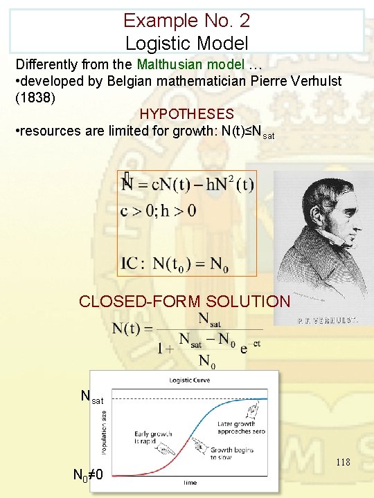
Example No. 2 Logistic Model Differently from the Malthusian model … • developed by Belgian mathematician Pierre Verhulst (1838) HYPOTHESES • resources are limited for growth: N(t)≤Nsat GENERAL CONSERVATION LAW applied to No. of individuals in a “closed system”: ACC = GEN GEN = birth - death STATE VARIABLES PARAMETERS CLASSIFICATION Dynamic autonomous mathematical model made by 1 ODE (Order =1) , non linear, constant coefficient model 24

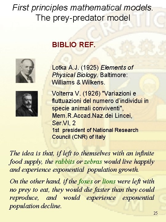
First principles mathematical models. The prey-predator model BIBLIO REF. Lotka A. J. (1925) Elements of Physical Biology. Baltimore: Williams & Wilkens. Volterra V. (1926) "Variazioni e fluttuazioni del numero d’individui in specie animali conviventi", Mem. R. Accad. Naz. dei Lincei, Ser. VI, 2 1 st president of National Research Council (CNR) of Italy The idea is that, if left to themselves with an infinite food supply, the rabbits or zebras would live happily and experience exponential population growth. On the other hand, if the foxes or lions were left with no prey to eat, they would die faster than they could reproduce, and would experience exponential population decline. 25

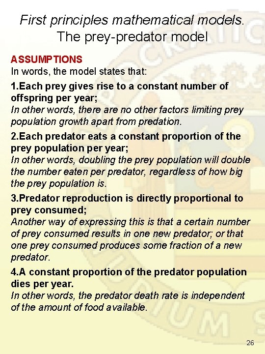
First principles mathematical models. The prey-predator model ASSUMPTIONS In words, the model states that: 1. Each prey gives rise to a constant number of offspring per year; In other words, there are no other factors limiting prey population growth apart from predation. 2. Each predator eats a constant proportion of the prey population per year; In other words, doubling the prey population will double the number eaten per predator, regardless of how big the prey population is. 3. Predator reproduction is directly proportional to prey consumed; Another way of expressing this is that a certain number of prey consumed results in one new predator; or that one prey consumed produces some fraction of a new predator. 4. A constant proportion of the predator population dies per year. In other words, the predator death rate is independent of the amount of food available. 26

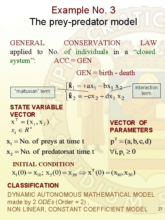
Example No. 3 The prey-predator model GENERAL CONSERVATION LAW applied to No. of individuals in a “closed system”: ACC = GEN = birth - death “maltusian” term interaction term STATE VARIABLE VECTOR OF PARAMETERS INITIAL CONDITION CLASSIFICATION DYNAMIC AUTONOMOUS MATHEMATICAL MODEL made by 2 ODEs (Order = 2) , NON LINEAR, CONSTANT COEFFICIENT MODEL 27

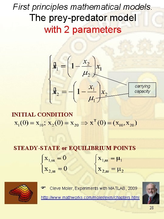
First principles mathematical models. The prey-predator model with 2 parameters carrying capacity INITIAL CONDITION STEADY-STATE or EQUILIBRIUM POINTS Cleve Moler, Experiments with MATLAB, 2009 http: //www. mathworks. com/moler/exm/chapters. html 28

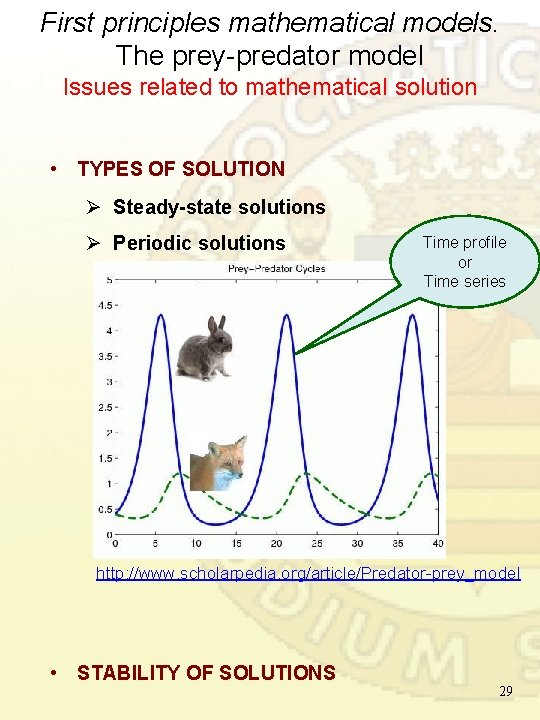
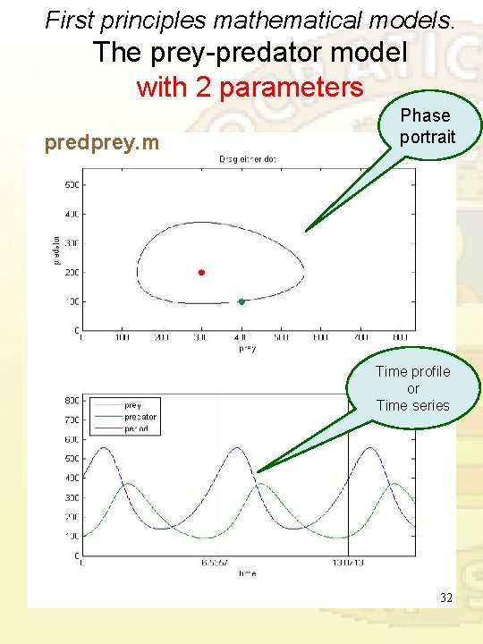
First principles mathematical models. The prey-predator model Issues related to mathematical solution • TYPES OF SOLUTION Ø Steady-state solutions Ø Periodic solutions Time profile or Time series http: //www. scholarpedia. org/article/Predator-prey_model • STABILITY OF SOLUTIONS 29

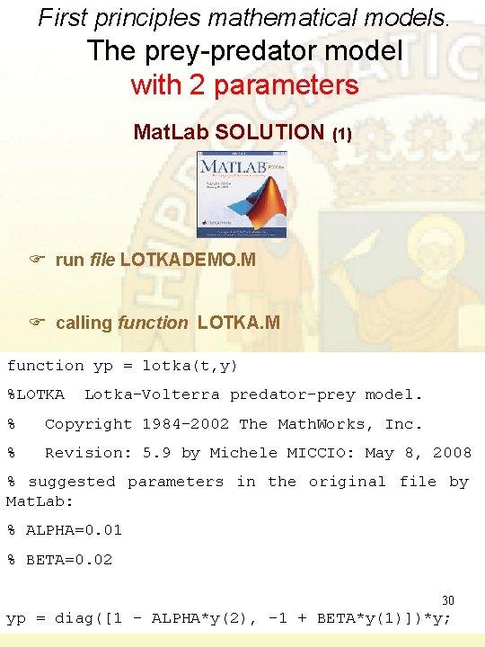
First principles mathematical models. The prey-predator model with 2 parameters Mat. Lab SOLUTION (1) run file LOTKADEMO. M calling function LOTKA. M function yp = lotka(t, y) %LOTKA Lotka-Volterra predator-prey model. % Copyright 1984 -2002 The Math. Works, Inc. % Revision: 5. 9 by Michele MICCIO: May 8, 2008 % suggested parameters in the original file by Mat. Lab: % ALPHA=0. 01 % BETA=0. 02 30 yp = diag([1 - ALPHA*y(2), -1 + BETA*y(1)])*y;

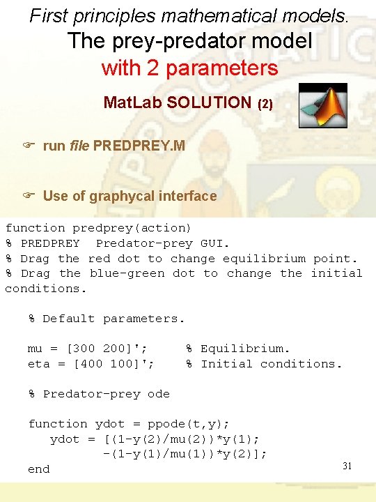
First principles mathematical models. The prey-predator model with 2 parameters Mat. Lab SOLUTION (2) run file PREDPREY. M Use of graphycal interface function predprey(action) % PREDPREY Predator-prey GUI. % Drag the red dot to change equilibrium point. % Drag the blue-green dot to change the initial conditions. % Default parameters. mu = [300 200]'; eta = [400 100]'; % Equilibrium. % Initial conditions. % Predator-prey ode function ydot = ppode(t, y); ydot = [(1 -y(2)/mu(2))*y(1); -(1 -y(1)/mu(1))*y(2)]; end 31

First principles mathematical models. The prey-predator model with 2 parameters predprey. m Phase portrait Time profile or Time series 32

Mathematical Models 1 st classification (on the base of the approach adopted for model development) ] “First principles Models” Basic models Models involving transport phenomena Models based on the “population balance approach” Empirical or “fitting” models ] Dynamic models ] • dynamic models with “input-output representation” • state-space dynamic models • black box dynamic models Time Series ] Statistical models ] rielaborated from § 1. 4 in Himmelblau D. M. e Bischoff K. B. , “Process Analysis and Simulation”, Wiley & Sons Inc. , 1967 33

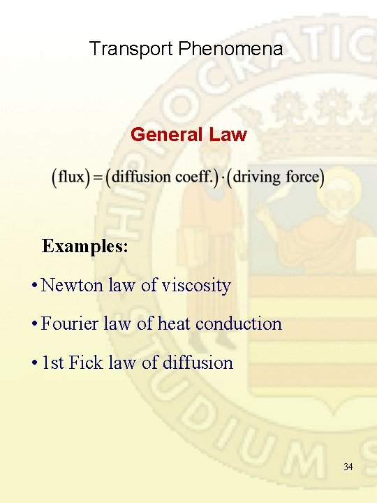
Transport Phenomena General Law Examples: • Newton law of viscosity • Fourier law of heat conduction • 1 st Fick law of diffusion 34

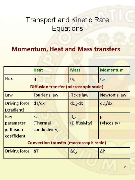
Transport and Kinetic Rate Equations Momentum, Heat and Mass transfers Flux Heat Mass Momentum q n. A τxy Diffusion transfer (microscopic scale) Law Fourier’s law Fick’s law Newton’s law Driving force d. T/dx d. CA/dx dvy/dx (gradient) Key k. T DAB µ parameter (Thermal (Diffusivity) (Viscosity) (diffusion conductivity) coefficient) Convection transfer (macroscopic scale) Driving force ∆T ∆CA ∆P 35

Mathematical Models 1 st classification (on the base of the approach adopted for model development) ] “First principle Models” Basic models Models involving trasport phenomena Models based on the “population balance approach” Empirical or “fitting” models ] Dynamic models ] • dynamic models with “input-output rappresentation” • state-space dynamic models • black box dynamic models Time Series ] Statistical models ] rielaborated from § 1. 4 in Himmelblau D. M. e Bischoff K. B. , “Process Analysis and Simulation”, Wiley & Sons Inc. , 1967 36

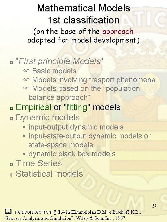
Mathematical Models 1 st classification (on the base of the approach adopted for model development) ] “First principle Models” Basic models Models involving trasport phenomena Models based on the “population balance approach” Empirical or “fitting” models ] Dynamic models ] • input-output dynamic models • input-state-output dynamic models or state-space models • dynamic black box models Time Series ] Statistical models ] rielaborated from § 1. 4 in Himmelblau D. M. e Bischoff K. B. , “Process Analysis and Simulation”, Wiley & Sons Inc. , 1967 37

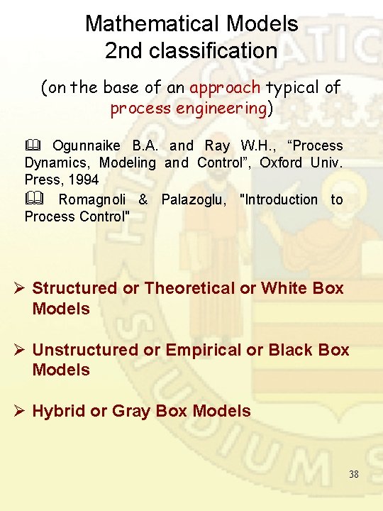
Mathematical Models 2 nd classification (on the base of an approach typical of process engineering) Ogunnaike B. A. and Ray W. H. , “Process Dynamics, Modeling and Control”, Oxford Univ. Press, 1994 Romagnoli & Palazoglu, "Introduction to Process Control" Ø Structured or Theoretical or White Box Models Ø Unstructured or Empirical or Black Box Models Ø Hybrid or Gray Box Models 38

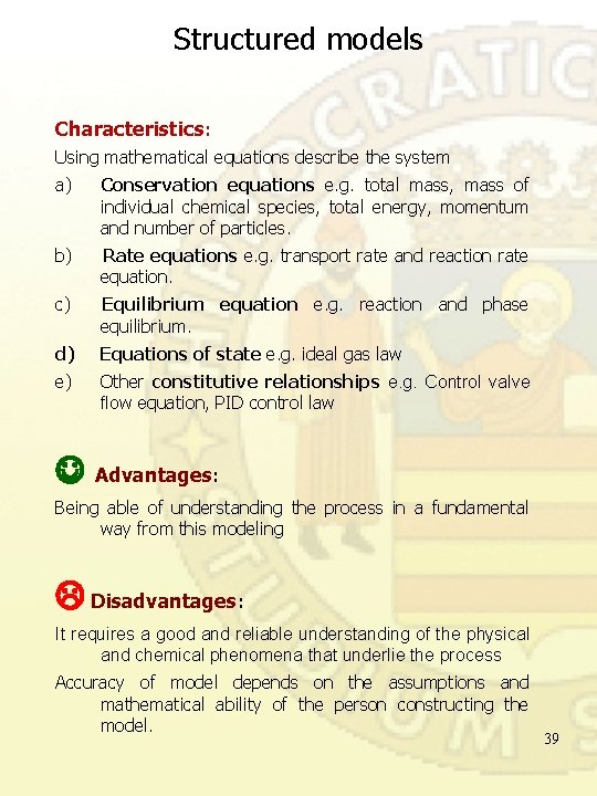
Structured models Characteristics: Using mathematical equations describe the system a) Conservation equations e. g. total mass, mass of individual chemical species, total energy, momentum and number of particles. b) Rate equations e. g. transport rate and reaction rate equation. c) Equilibrium equation e. g. reaction and phase equilibrium. d) Equations of state e. g. ideal gas law e) Other constitutive relationships e. g. Control valve flow equation, PID control law Advantages: Being able of understanding the process in a fundamental way from this modeling Disadvantages: It requires a good and reliable understanding of the physical and chemical phenomena that underlie the process Accuracy of model depends on the assumptions and mathematical ability of the person constructing the model. 39

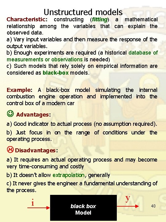
Unstructured models Characteristic: constructing (fitting) a mathematical relationship among the variables that can explain the observed data. a) Vary input variables and then measure the response of the output variables. b) Enough experiments are required (a historical database of measurements or observations is needed) c) Such models that rely solely on empirical information are considered as black-box models. Example: A black-box model simulating the internal combustion engine operation and implemented into the control box of a modern car Advantages: a) Good indicator to actual process (no assumption required). b) Just focus in on the range of conditions under the operating process. Disadvantages: a) It requires an actual operating process and may become very time-consuming and costly b) It doesn’t allow extrapolation, generally c) It never gives the engineer a fundamental understanding of the process. i y black box Model 40

Structured and un. Structured Models: Comparison Structured Models theory-rich and data-poor Unstructured Models data-rich and theory-poor 41

“Hybrid” Models • Empirical Model II (Gray-Box) is developed by incorporating empirical knowledge into the fundamental understanding of the process. Such models blending fundamental and empirical knowledge are referred to as gray -box models. Example An example can be the use of mass and energy balances to develop a reactor model and the rate of the reaction will be based on expressions obtained from laboratory experiments. 42 Introduction to Process Control Romagnoli & Palazoglu

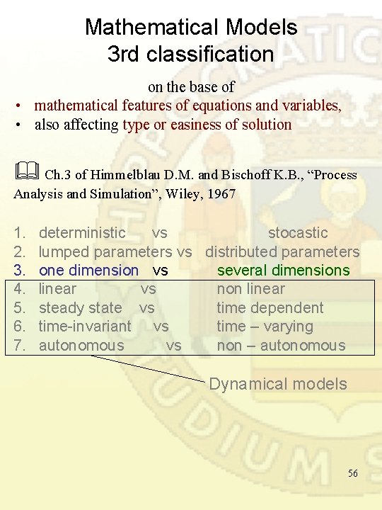
Mathematical Models 3 rd classification on the base of • mathematical features of equations and variables, • also affecting type or easiness of solution Ch. 3 of Himmelblau D. M. and Bischoff K. B. , “Process Analysis and Simulation”, Wiley, 1967 1. 2. 3. 4. 5. 6. 7. deterministic vs stocastic lumped parameters vs distributed parameters one dimension vs several dimensions linear vs non linear steady state vs time dependent time-invariant vs time – varying autonomous vs non – autonomous Dynamical models 43

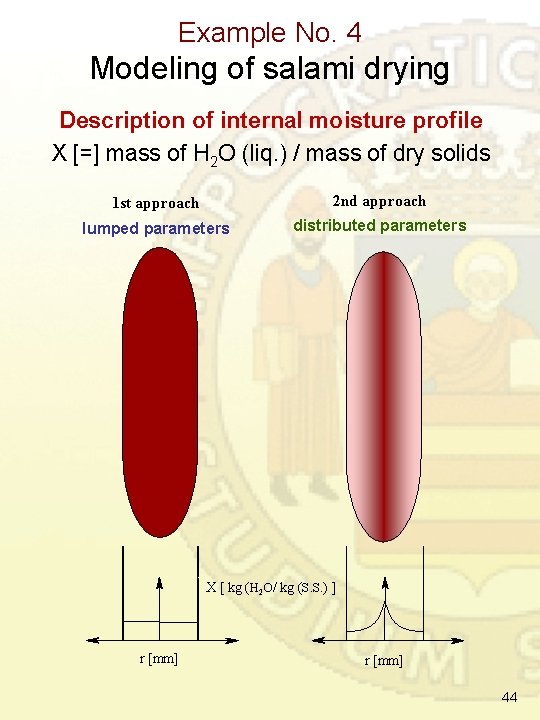
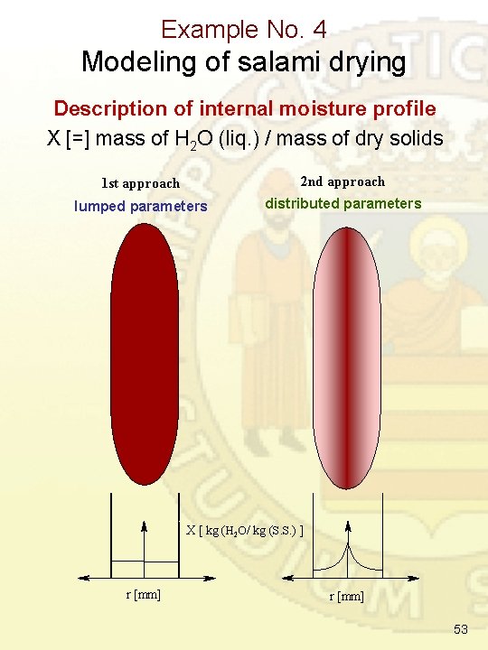
Example No. 4 Modeling of salami drying Description of internal moisture profile X [=] mass of H 2 O (liq. ) / mass of dry solids 1 st approach 2 nd approach lumped parameters distributed parameters X [ kg (H 2 O/ kg (S. S. ) ] r [mm] 44

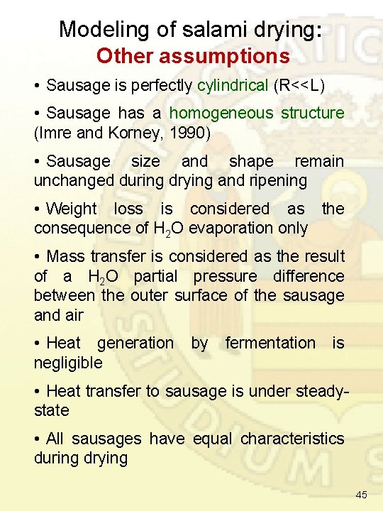
Modeling of salami drying: Other assumptions • Sausage is perfectly cylindrical (R<<L) • Sausage has a homogeneous structure (Imre and Korney, 1990) • Sausage size and shape remain unchanged during drying and ripening • Weight loss is considered as the consequence of H 2 O evaporation only • Mass transfer is considered as the result of a H 2 O partial pressure difference between the outer surface of the sausage and air • Heat generation by fermentation is negligible • Heat transfer to sausage is under steadystate • All sausages have equal characteristics during drying 45

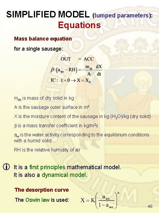
SIMPLIFIED MODEL (lumped parameters): Equations Mass balance equation for a single sausage: mds is mass of dry solid in kg A is the sausage outer surface in m² X is the moisture content of the sausage in kg (H 2 O)/kg (dry solid) is a mass transfer coefficient in kg/m 2 s aw is the water activity corresponding to the equilibrium conditions with a humid solid RH is the relative humidity of air It is a first principles mathematical model. It is also a dynamical model. The desorption curve The Oswin law is used: 46

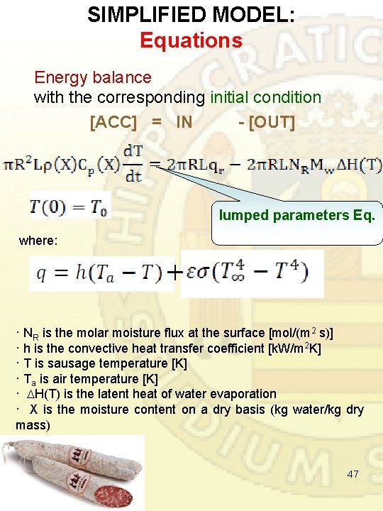
SIMPLIFIED MODEL: Equations Energy balance with the corresponding initial condition [ACC] = IN - [OUT] lumped parameters Eq. where: · NR is the molar moisture flux at the surface [mol/(m 2 s)] · h is the convective heat transfer coefficient [k. W/m 2 K] · T is sausage temperature [K] · Ta is air temperature [K] · H(T) is the latent heat of water evaporation · X is the moisture content on a dry basis (kg water/kg dry mass) 47

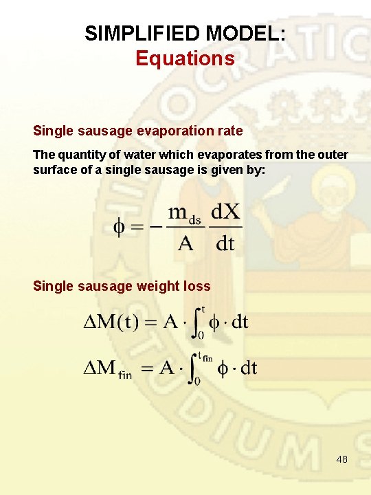
SIMPLIFIED MODEL: Equations Single sausage evaporation rate The quantity of water which evaporates from the outer surface of a single sausage is given by: Single sausage weight loss 48

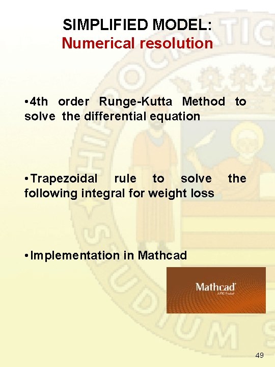
SIMPLIFIED MODEL: Numerical resolution • 4 th order Runge-Kutta Method to solve the differential equation • Trapezoidal rule to solve following integral for weight loss the • Implementation in Mathcad 49

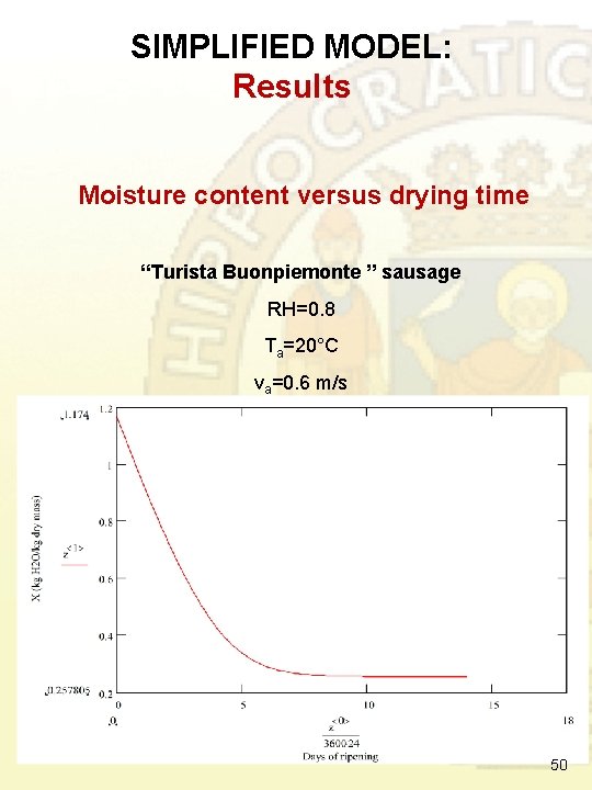
SIMPLIFIED MODEL: Results Moisture content versus drying time “Turista Buonpiemonte ” sausage RH=0. 8 Ta=20°C va=0. 6 m/s 50

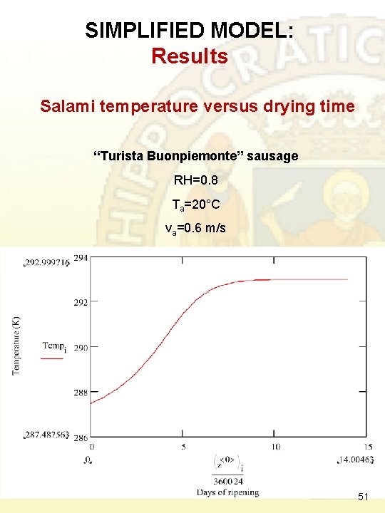
SIMPLIFIED MODEL: Results Salami temperature versus drying time “Turista Buonpiemonte” sausage RH=0. 8 Ta=20°C va=0. 6 m/s 51

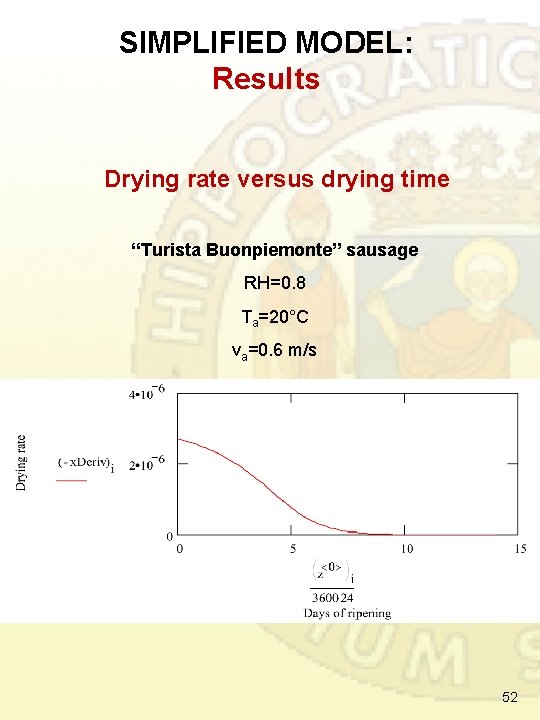
SIMPLIFIED MODEL: Results Drying rate versus drying time “Turista Buonpiemonte” sausage RH=0. 8 Ta=20°C va=0. 6 m/s 52

Example No. 4 Modeling of salami drying Description of internal moisture profile X [=] mass of H 2 O (liq. ) / mass of dry solids 1 st approach 2 nd approach lumped parameters distributed parameters X [ kg (H 2 O/ kg (S. S. ) ] r [mm] 53

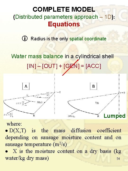
COMPLETE MODEL (Distributed parameters approach – 1 D): Equations Radius is the only spatial coordinate Water mass balance in a cylindrical shell [IN] – [OUT] + [GEN] = [ACC] Lumped where: D(X, T) is the mass diffusion coefficient depending on sausage moisture content and on sausage temperature (m 2/s) X is the moisture content on a dry basis (kg water/kg dry mass) 54

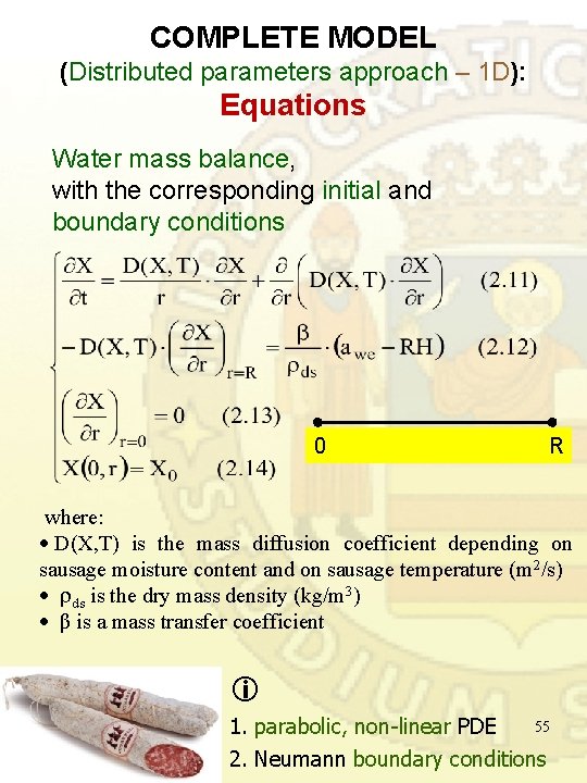
COMPLETE MODEL (Distributed parameters approach – 1 D): Equations Water mass balance, with the corresponding initial and boundary conditions 0 R where: D(X, T) is the mass diffusion coefficient depending on sausage moisture content and on sausage temperature (m 2/s) ds is the dry mass density (kg/m 3) β is a mass transfer coefficient 1. parabolic, non-linear PDE 55 2. Neumann boundary conditions

Mathematical Models 3 rd classification on the base of • mathematical features of equations and variables, • also affecting type or easiness of solution Ch. 3 of Himmelblau D. M. and Bischoff K. B. , “Process Analysis and Simulation”, Wiley, 1967 1. 2. 3. 4. 5. 6. 7. deterministic vs stocastic lumped parameters vs distributed parameters one dimension vs several dimensions linear vs non linear steady state vs time dependent time-invariant vs time – varying autonomous vs non – autonomous Dynamical models 56

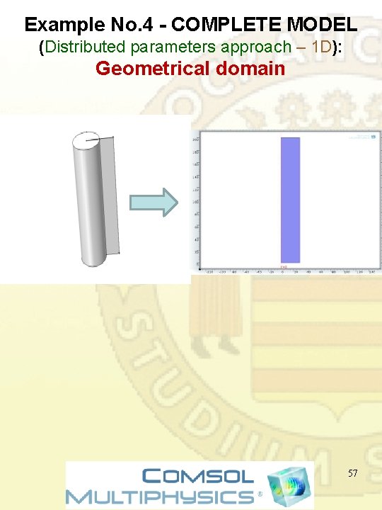
Example No. 4 - COMPLETE MODEL (Distributed parameters approach – 1 D): Geometrical domain 57

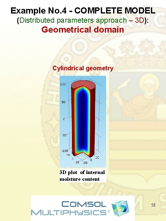
Example No. 4 - COMPLETE MODEL (Distributed parameters approach – 3 D): Geometrical domain Cylindrical geometry 3 D plot of internal moisture content 58

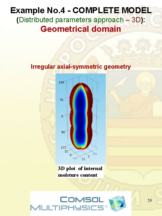
Example No. 4 - COMPLETE MODEL (Distributed parameters approach – 3 D): Geometrical domain Irregular axial-symmetric geometry 3 D plot of internal moisture content 59

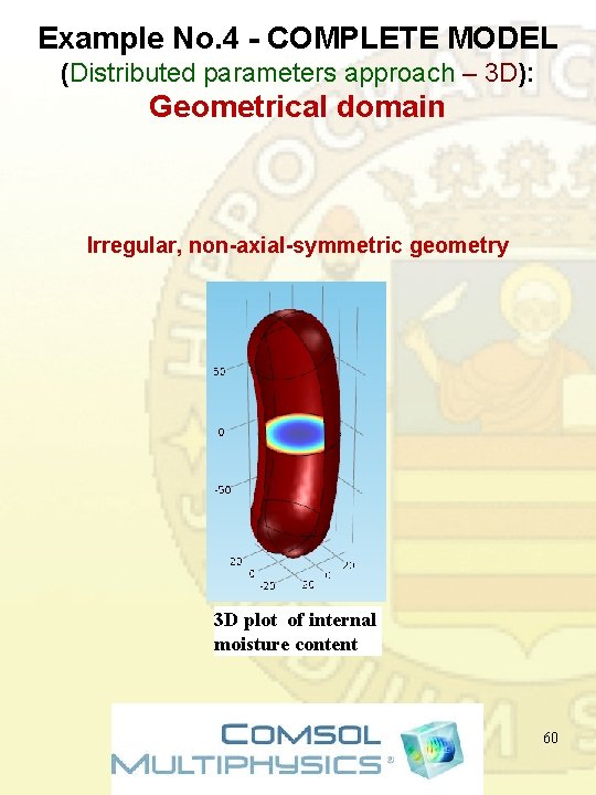
Example No. 4 - COMPLETE MODEL (Distributed parameters approach – 3 D): Geometrical domain Irregular, non-axial-symmetric geometry 3 D plot of internal moisture content 60

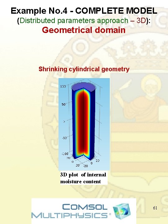
Example No. 4 - COMPLETE MODEL (Distributed parameters approach – 3 D): Geometrical domain Shrinking cylindrical geometry 3 D plot of internal moisture content 61

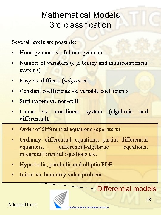
Mathematical Models 3 rd classification Several levels are possible: • Homogeneous vs. Inhomogeneous • Number of variables (e. g. binary and multicomponent systems) • Easy vs. difficult (subjective) • Constant coefficients vs. variable coefficients • Stiff system vs. non-stiff • Linear vs. non-linear system (algebraic and differential). • Order of differential equations (operators) • Ordinary differential equations, partial differential equations, differential-algebraic equations, integrodifferential equations etc. • Hyperbolic, parabolic and elliptic PDE • Initial vs. boundary value problem Differential models 62 Adapted from: TEKNILLINEN KORKEAKOULU

Mathematical Models 3 rd classification Homogeneous vs. inhomogeneous If f( x)= nf(x) for every , then f(x) is homogeneous to n: th degree. Number of variables • One-component system • Two-component system • Multi-component system More components, more degrees of freedom. Often one degree of freedom leads to scalar equations, more degrees to matrices. 63

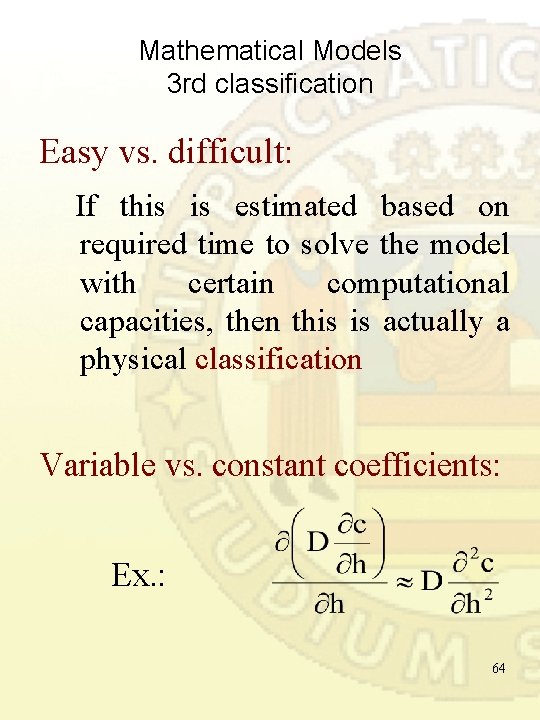
Mathematical Models 3 rd classification Easy vs. difficult: If this is estimated based on required time to solve the model with certain computational capacities, then this is actually a physical classification Variable vs. constant coefficients: Ex. : 64

Mathematical Models 3 rd classification Stiff vs. non-stiff – Formally, based on the ratio of eigenvalues – In practice, if there are simultaneously very fast phenomena dictating step sizes, and very slow phenomena dictating simulation time, system is stiff. Linear vs. non-linear In principle, linear systems are easy. Natural systems are rarely linear, but often numerical solution is based on (local) linearizations 65

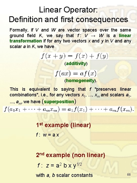
Linear Operator: Definition and first consequences Formally, if V and W are vector spaces over the same ground field K, we say that f : V → W is a linear transformation if for any two vectors x and y in V and any scalar a in K, we have (additivity) (homogeneity). This is equivalent to saying that f "preserves linear combinations", i. e. , for any vectors x 1, . . . , xm and scalars a 1, . . . , am, we have (superposition) 1 st example (linear) f : w = a x 2 nd example (non linear) f : z = a 2 b x y 1/2 with a, b scalar constants 66

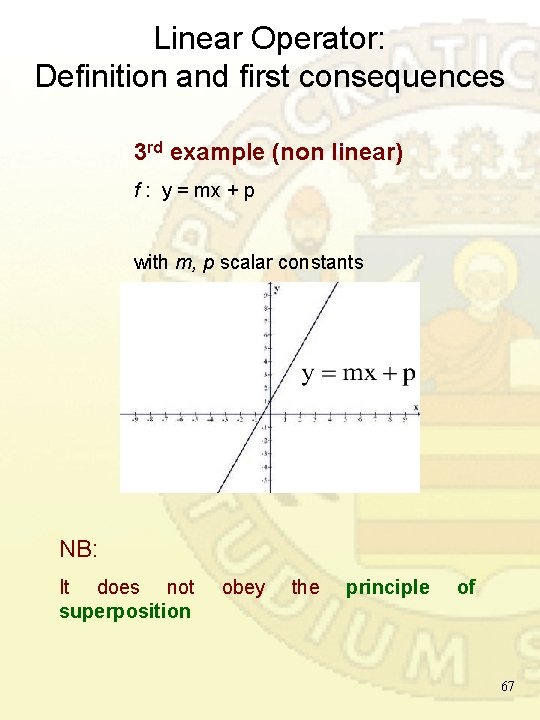
Linear Operator: Definition and first consequences 3 rd example (non linear) f : y = mx + p with m, p scalar constants NB: It does not superposition obey the principle of 67

Mathematical Models 3 rd classification Several levels are possible: • Homogeneous vs. Inhomogeneous • Number of variables (e. g. binary and multicomponent systems) • Easy vs. difficult (subjective) • Constant coefficients vs. variable coefficients • Stiff system vs. non-stiff • Linear vs. non-linear system (algebraic and differential). • Order of differential equations (operators) • Ordinary differential equations, partial differential equations, differential-algebraic equations, integrodifferential equations etc. • Hyperbolic, parabolic and elliptic PDE • Initial vs. boundary value problem Differential models 68 Adapted from: TEKNILLINEN KORKEAKOULU

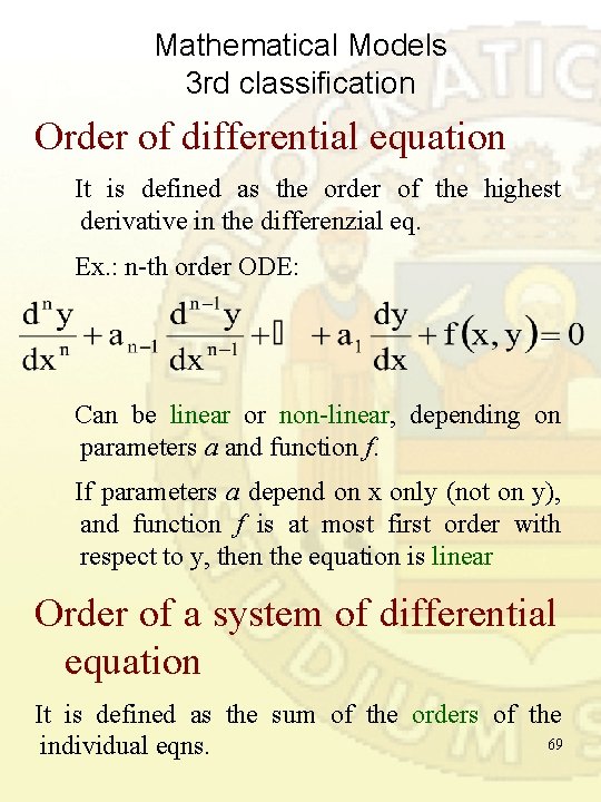
Mathematical Models 3 rd classification Order of differential equation It is defined as the order of the highest derivative in the differenzial eq. Ex. : n-th order ODE: Can be linear or non-linear, depending on parameters a and function f. If parameters a depend on x only (not on y), and function f is at most first order with respect to y, then the equation is linear Order of a system of differential equation It is defined as the sum of the orders of the 69 individual eqns.

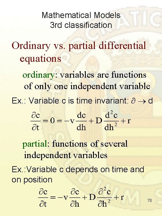
Mathematical Models 3 rd classification Ordinary vs. partial differential equations ordinary: variables are functions of only one independent variable Ex. : Variable c is time invariant: d partial: functions of several independent variables Ex. : Variable c depends on time and on position 70

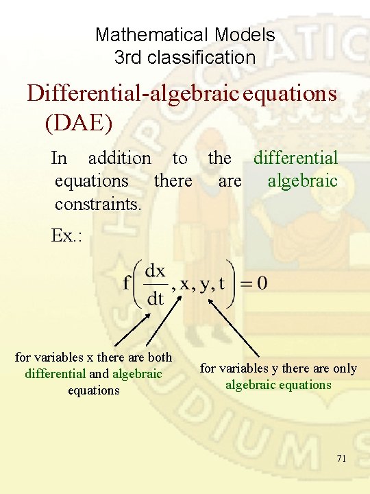
Mathematical Models 3 rd classification Differential-algebraic equations (DAE) In addition to the differential equations there algebraic constraints. Ex. : for variables x there are both differential and algebraic equations for variables y there are only algebraic equations 71

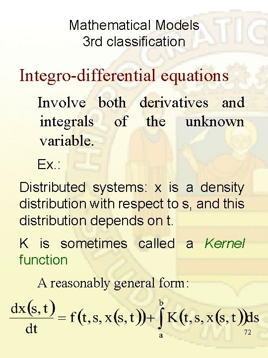
Mathematical Models 3 rd classification Integro-differential equations Involve both derivatives and integrals of the unknown variable. Ex. : Distributed systems: x is a density distribution with respect to s, and this distribution depends on t. K is sometimes called a Kernel function A reasonably general form: 72

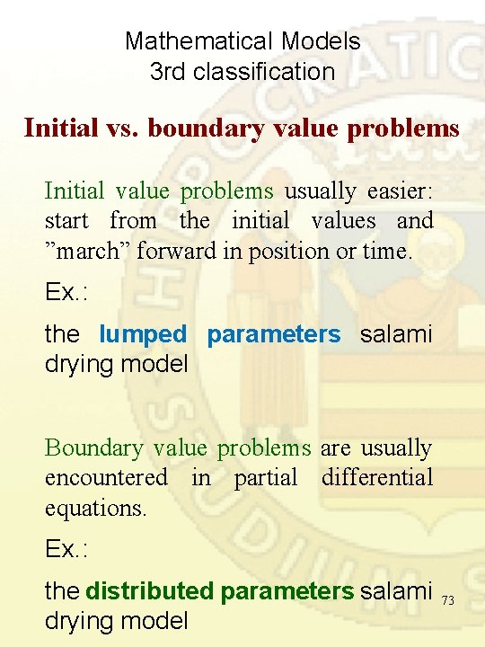
Mathematical Models 3 rd classification Initial vs. boundary value problems Initial value problems usually easier: start from the initial values and ”march” forward in position or time. Ex. : the lumped parameters salami drying model Boundary value problems are usually encountered in partial differential equations. Ex. : the distributed parameters salami 73 drying model

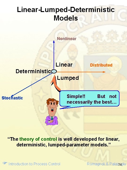
Linear-Lumped-Deterministic Models Nonlinear Linear Distributed Deterministic Lumped Stochastic Simple!! But not necessarily the best… “The theory of control is well developed for linear, deterministic, lumped-parameter models. ” Introduction to Process Control Romagnoli & Palazoglu 74

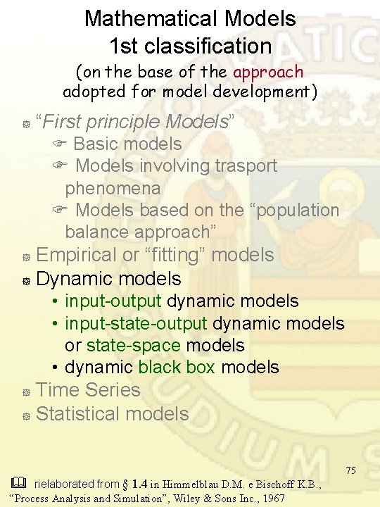
Mathematical Models 1 st classification (on the base of the approach adopted for model development) ] “First principle Models” Basic models Models involving trasport phenomena Models based on the “population balance approach” Empirical or “fitting” models ] Dynamic models ] • input-output dynamic models • input-state-output dynamic models or state-space models • dynamic black box models Time Series ] Statistical models ] rielaborated from § 1. 4 in Himmelblau D. M. e Bischoff K. B. , “Process Analysis and Simulation”, Wiley & Sons Inc. , 1967 75

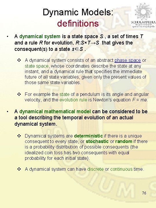
Dynamic Models: definitions • A dynamical system is a state space S , a set of times T and a rule R for evolution, R: S×T→S that gives the consequent(s) to a state s∈S. v A dynamical system consists of an abstract phase space or state space, whose coordinates describe the state at any instant, and a dynamical rule that specifies the immediate future of all state variables, given only the present values of those same state variables. v For example the state of a pendulum is its angle and angular velocity, and the evolution rule is Newton's equation F = ma. • A dynamical mathematical model can be considered to be a tool describing the temporal evolution of an actual dynamical system. v Dynamical systems are deterministic if there is a unique consequent to every state, or stochastic or random if there is a probability distribution of possible consequents (the idealized coin toss has two consequents with equal probability for each initial state). v A dynamical system can have discrete or continuous time. 76

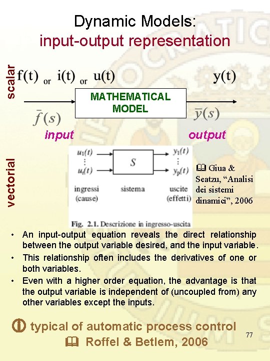
scalar Dynamic Models: input-output representation MATHEMATICAL MODEL vectorial input output Giua & Seatzu, “Analisi dei sistemi dinamici”, 2006 • An input-output equation reveals the direct relationship between the output variable desired, and the input variable. • This relationship often includes the derivatives of one or both variables. • Even with a higher order equation, the advantage is that the output variable is independent of (uncoupled from) any other variables except the inputs. typical of automatic process control Roffel & Betlem, 2006 77

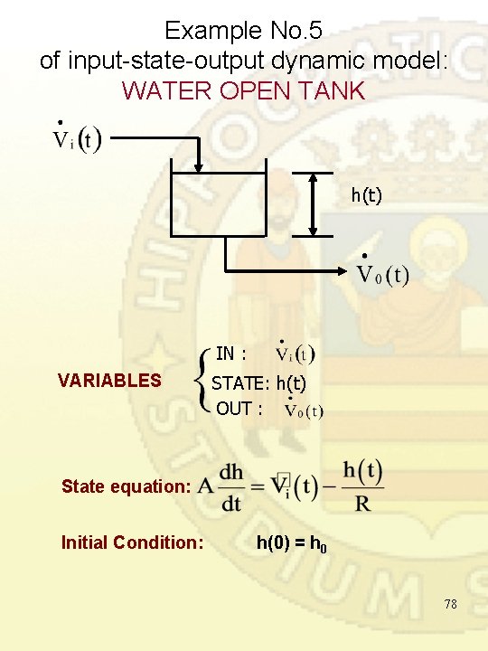
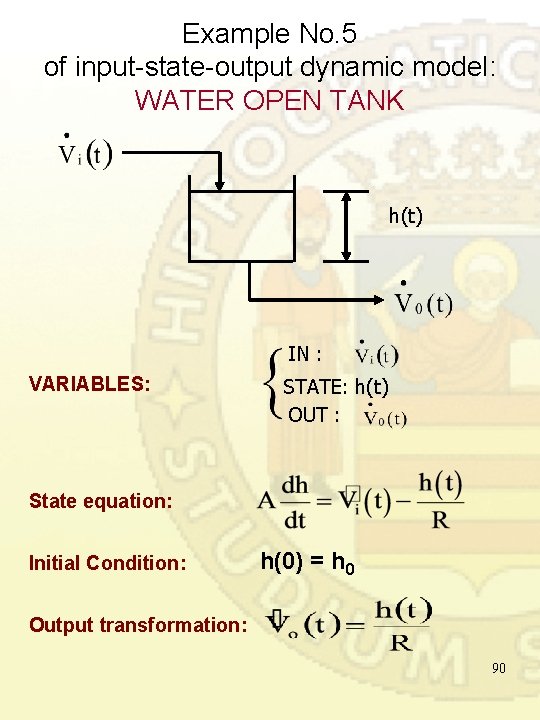
Example No. 5 of input-state-output dynamic model: WATER OPEN TANK h(t) IN : VARIABLES STATE: h(t) OUT : State equation: Initial Condition: h(0) = h 0 78

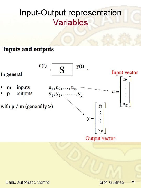
Input-Output representation Variables Basic Automatic Control prof. Guariso 79

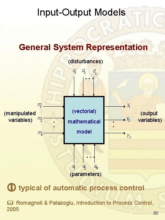
Input-Output Models General System Representation (disturbances) d 1 m 1 (manipulated variables) m 2 d. L … y 1 (vectorial) : mathematical Process model m. K : y 2 (output variables) y. J … a 1 a 2 a. R (parameters) typical of automatic process control Romagnoli & Palazoglu, Introduction to Process Control, 2005 80

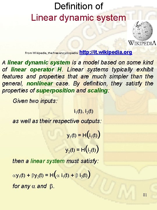
Definition of Linear dynamic system From Wikipedia, the free encyclopedia: http: //it. wikipedia. org A linear dynamic system is a model based on some kind of linear operator H. Linear systems typically exhibit features and properties that are much simpler than the general, nonlinear case. By definition, they satisfy the properties of superposition and scaling: Given two inputs: i 1(t), i 2(t) as well as their respective outputs: ( ) y 1(t) = H i 1(t) ( ) y 2(t) = H i 2(t) then a linear system must satisfy: ( y 1(t) + y 2(t) = H i 1(t) + i 2(t) ) for any and . 81

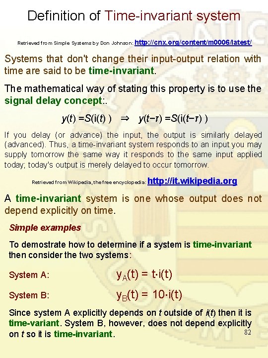
Definition of Time-invariant system Retrieved from Simple Systems by Don Johnson: http: //cnx. org/content/m 0006/latest/ Systems that don't change their input-output relation with time are said to be time-invariant. The mathematical way of stating this property is to use the signal delay concept: . y(t) =S(i(t) ) ⇒ y(t−τ) =S(i(t−τ) ) If you delay (or advance) the input, the output is similarly delayed (advanced). Thus, a time-invariant system responds to an input you may supply tomorrow the same way it responds to the same input applied today; today's output is merely delayed to occur tomorrow. Retrieved from Wikipedia, the free encyclopedia: http: //it. wikipedia. org A time-invariant system is one whose output does not depend explicitly on time. Simple examples To demostrate how to determine if a system is time-invariant then consider the two systems: System A: y. A(t) = t i(t) System B: y. B(t) = 10 i(t) Since system A explicitly depends on t outside of i(t) then it is time-variant. System B, however, does not depend explicitly 82 on t so it is time-invariant.

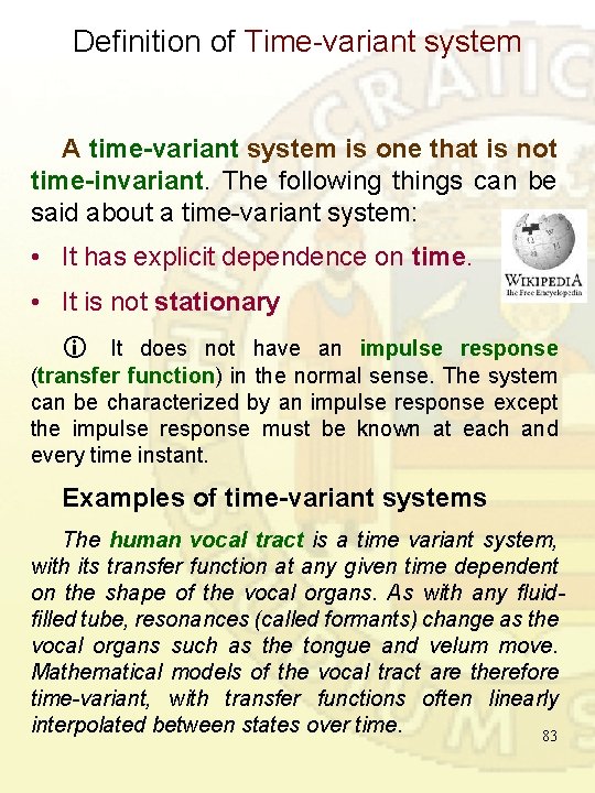
Definition of Time-variant system A time-variant system is one that is not time-invariant. The following things can be said about a time-variant system: • It has explicit dependence on time. • It is not stationary It does not have an impulse response (transfer function) in the normal sense. The system can be characterized by an impulse response except the impulse response must be known at each and every time instant. Examples of time-variant systems The human vocal tract is a time variant system, with its transfer function at any given time dependent on the shape of the vocal organs. As with any fluidfilled tube, resonances (called formants) change as the vocal organs such as the tongue and velum move. Mathematical models of the vocal tract are therefore time-variant, with transfer functions often linearly interpolated between states over time. 83

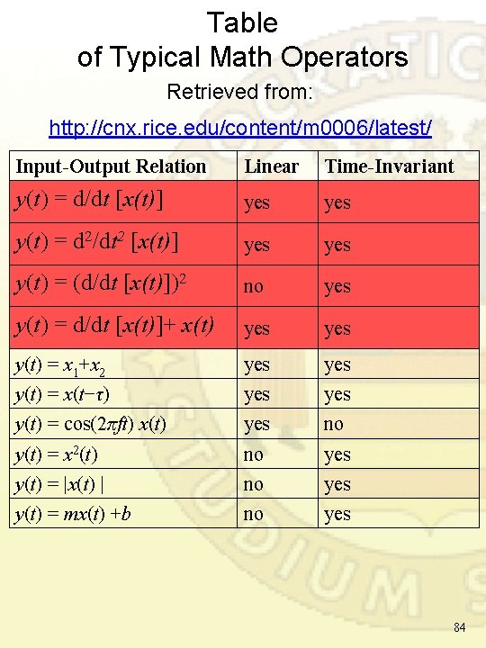
Table of Typical Math Operators Retrieved from: http: //cnx. rice. edu/content/m 0006/latest/ Input-Output Relation Linear Time-Invariant y(t) = d/dt [x(t)] yes y(t) = d 2/dt 2 [x(t)] yes y(t) = (d/dt [x(t)])2 no yes y(t) = d/dt [x(t)]+ x(t) yes y(t) = x 1+x 2 yes y(t) = x(t−τ) yes y(t) = cos(2πft) x(t) yes no y(t) = x 2(t) no yes y(t) = |x(t) | no yes y(t) = mx(t) +b no yes 84

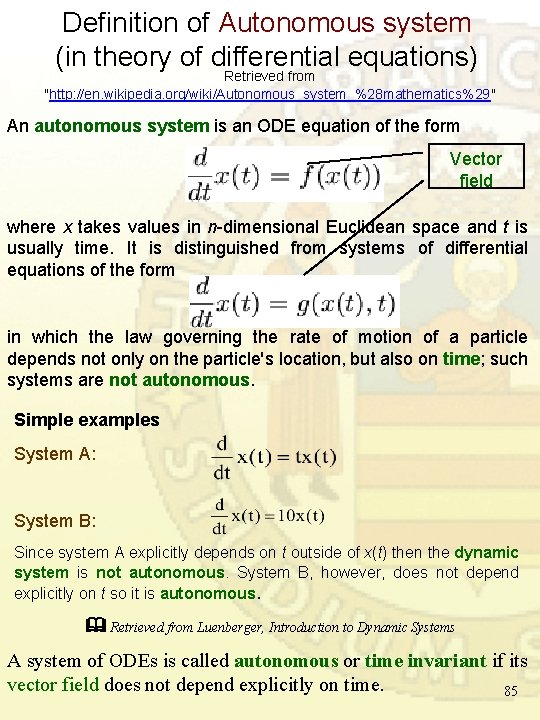
Definition of Autonomous system (in theory of differential equations) Retrieved from "http: //en. wikipedia. org/wiki/Autonomous_system_%28 mathematics%29" An autonomous system is an ODE equation of the form Vector field where x takes values in n-dimensional Euclidean space and t is usually time. It is distinguished from systems of differential equations of the form in which the law governing the rate of motion of a particle depends not only on the particle's location, but also on time; such systems are not autonomous. Simple examples System A: System B: Since system A explicitly depends on t outside of x(t) then the dynamic system is not autonomous. System B, however, does not depend explicitly on t so it is autonomous. Retrieved from Luenberger, Introduction to Dynamic Systems A system of ODEs is called autonomous or time invariant if its vector field does not depend explicitly on time. 85

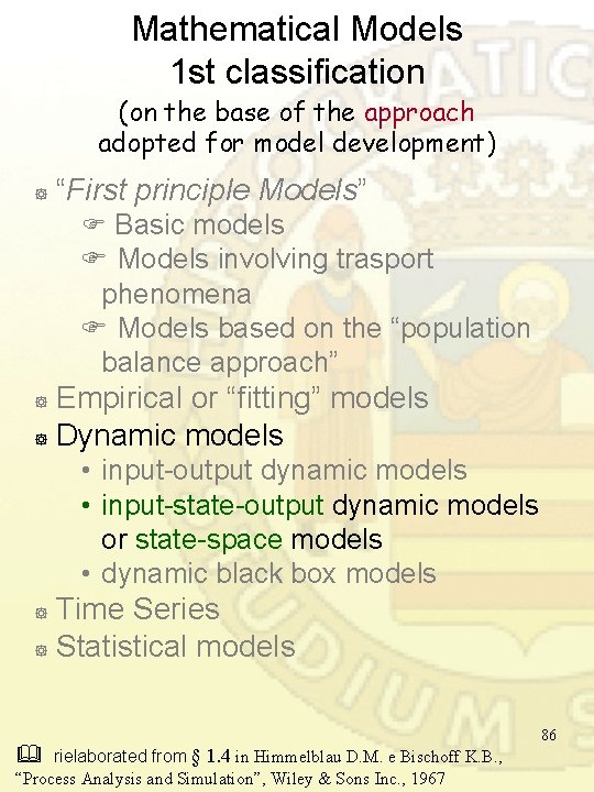
Mathematical Models 1 st classification (on the base of the approach adopted for model development) ] “First principle Models” Basic models Models involving trasport phenomena Models based on the “population balance approach” Empirical or “fitting” models ] Dynamic models ] • input-output dynamic models • input-state-output dynamic models or state-space models • dynamic black box models Time Series ] Statistical models ] rielaborated from § 1. 4 in Himmelblau D. M. e Bischoff K. B. , “Process Analysis and Simulation”, Wiley & Sons Inc. , 1967 86

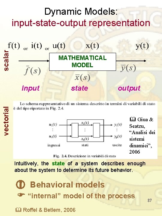
scalar Dynamic Models: input-state-output representation MATHEMATICAL MODEL state vectorial Input output Giua & Seatzu, “Analisi dei sistemi dinamici”, 2006 Intuitively, the state of a system describes enough about the system to determine its future behavior. Behavioral models “internal” model of the process Roffel & Betlem, 2006 87

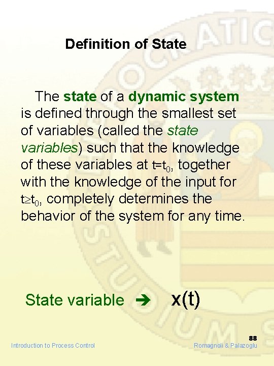
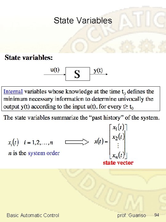
Definition of State The state of a dynamic system is defined through the smallest set of variables (called the state variables) such that the knowledge of these variables at t=t 0, together with the knowledge of the input for t t 0, completely determines the behavior of the system for any time. State variable Introduction to Process Control x(t) 88 Romagnoli & Palazoglu

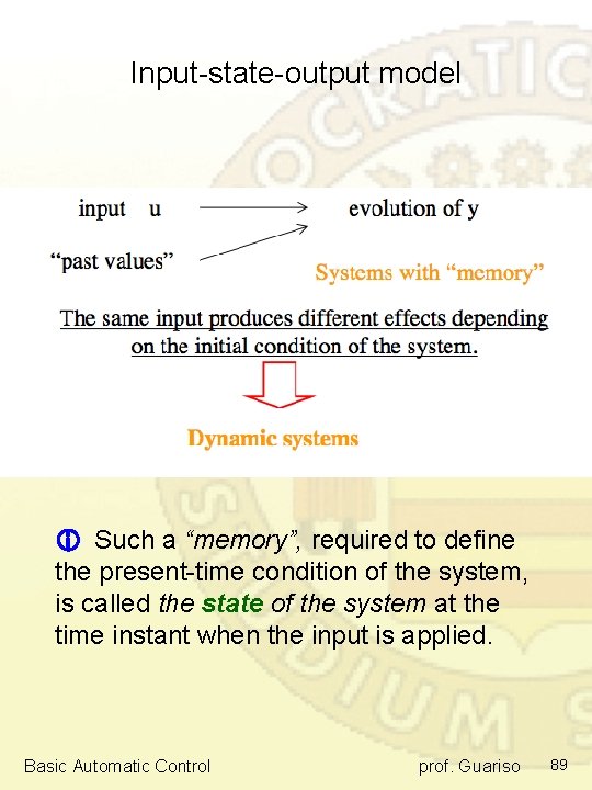
Input-state-output model Such a “memory”, required to define the present-time condition of the system, is called the state of the system at the time instant when the input is applied. Basic Automatic Control prof. Guariso 89

Example No. 5 of input-state-output dynamic model: WATER OPEN TANK h(t) IN : VARIABLES: STATE: h(t) OUT : State equation: Initial Condition: h(0) = h 0 Output transformation: 90

VARIABLES Variables are things that vary and change 91

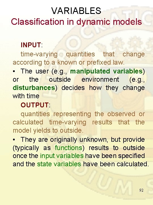
VARIABLES Classification in dynamic models INPUT: time-varying quantities that change according to a known or prefixed law. • The user (e. g. , manipulated variables) or the outside environment (e. g. , disturbances) decides how they change with time OUTPUT: quantities representing the observed or calculated time-varying results that the model yields to outside. • They are originally unknown, but provide (typically as functions) results to outside once the input variables have been specified and the state variables have been calculated. 92

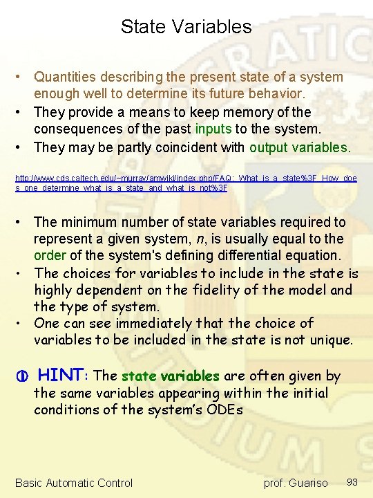
State Variables • Quantities describing the present state of a system enough well to determine its future behavior. • They provide a means to keep memory of the consequences of the past inputs to the system. • They may be partly coincident with output variables. http: //www. cds. caltech. edu/~murray/amwiki/index. php/FAQ: _What_is_a_state%3 F_How_doe s_one_determine_what_is_a_state_and_what_is_not%3 F • The minimum number of state variables required to represent a given system, n, is usually equal to the order of the system's defining differential equation. • The choices for variables to include in the state is highly dependent on the fidelity of the model and the type of system. • One can see immediately that the choice of variables to be included in the state is not unique. HINT: The state variables are often given by the same variables appearing within the initial conditions of the system’s ODEs Basic Automatic Control prof. Guariso 93

State Variables Basic Automatic Control prof. Guariso 94

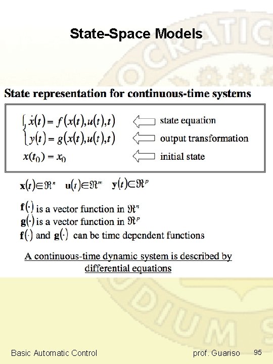
State-Space Models Basic Automatic Control prof. Guariso 95

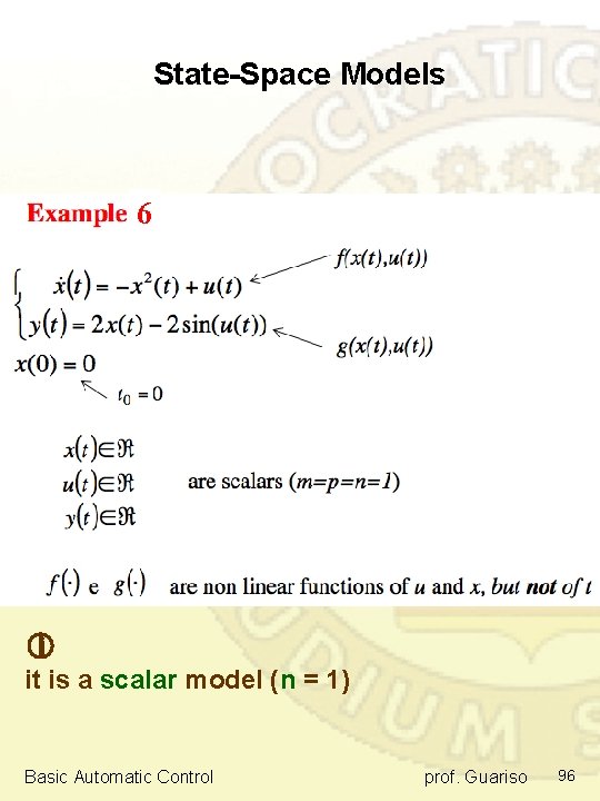
State-Space Models 6 it is a scalar model (n = 1) Basic Automatic Control prof. Guariso 96

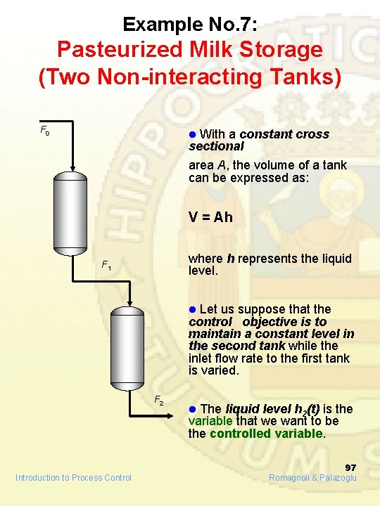
Example No. 7: Pasteurized Milk Storage (Two Non-interacting Tanks) F 0 l With a constant sectional cross area A, the volume of a tank can be expressed as: V = Ah where h represents the liquid level. F 1 l Let us suppose that the control objective is to maintain a constant level in the second tank while the inlet flow rate to the first tank is varied. F 2 Introduction to Process Control l The liquid level h 2(t) is the variable that we want to be the controlled variable. 97 Romagnoli & Palazoglu

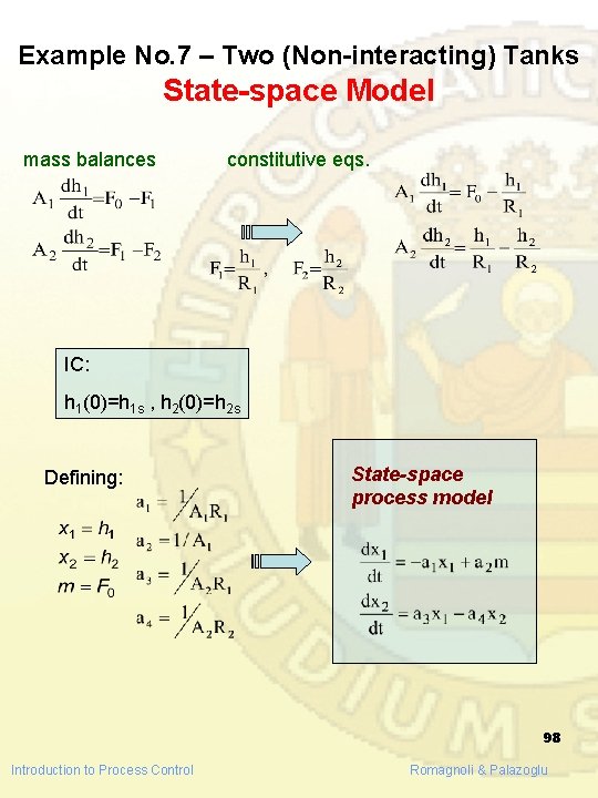
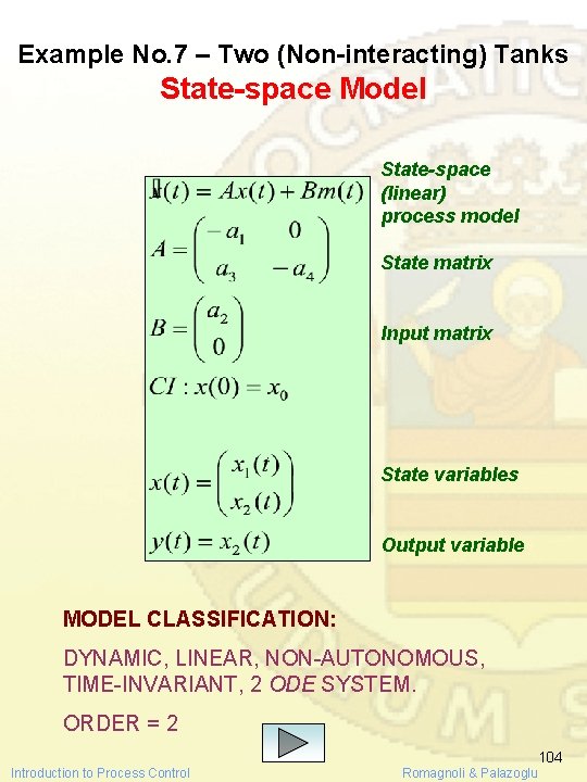
Example No. 7 – Two (Non-interacting) Tanks State-space Model mass balances constitutive eqs. IC: h 1(0)=h 1 s , h 2(0)=h 2 s Defining: State-space process model 98 Introduction to Process Control Romagnoli & Palazoglu

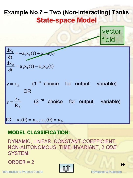
Example No. 7 – Two (Non-interacting) Tanks State-space Model vector field MODEL CLASSIFICATION: DYNAMIC, LINEAR, CONSTANT-COEFFICIENT, NON-AUTONOMOUS, TIME-INVARIANT, 2 ODE SYSTEM. ORDER = 2 Introduction to Process Control 99 Romagnoli & Palazoglu

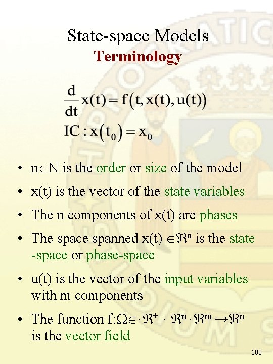
State-space Models Terminology • n N is the order or size of the model • x(t) is the vector of the state variables • The n components of x(t) are phases • The space spanned x(t) n is the state -space or phase-space • u(t) is the vector of the input variables with m components • The function f: · + · n · m → n is the vector field 100

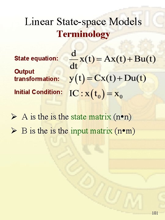
Linear State-space Models Terminology State equation: Output transformation: Initial Condition: Ø A is the state matrix (n n) Ø B is the input matrix (n m) 101

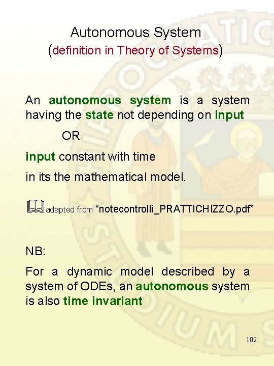
Autonomous System (definition in Theory of Systems) An autonomous system is a system having the state not depending on input OR input constant with time in its the mathematical model. adapted from “notecontrolli_PRATTICHIZZO. pdf” NB: For a dynamic model described by a system of ODEs, an autonomous system is also time invariant 102

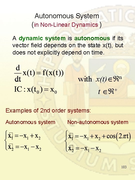
Autonomous System (in Non-Linear Dynamics ) A dynamic system is autonomous if its vector field depends on the state x(t), but does not explicitly depend on time. with x(t) n t + Examples of 2 nd order systems: Autonomous system Non-autonomous system 103

Example No. 7 – Two (Non-interacting) Tanks State-space Model State-space (linear) process model State matrix Input matrix State variables Output variable MODEL CLASSIFICATION: DYNAMIC, LINEAR, NON-AUTONOMOUS, TIME-INVARIANT, 2 ODE SYSTEM. ORDER = 2 Introduction to Process Control 104 Romagnoli & Palazoglu

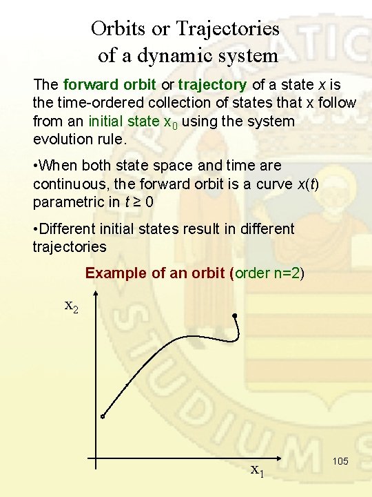
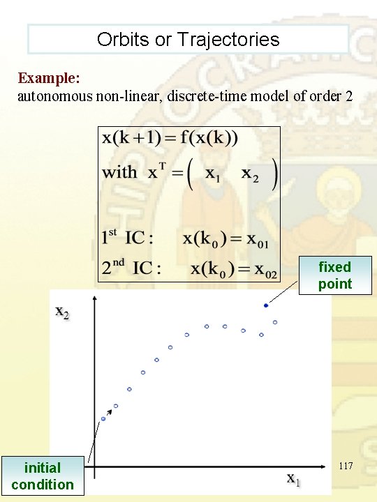
Orbits or Trajectories of a dynamic system The forward orbit or trajectory of a state x is the time-ordered collection of states that x follow from an initial state x 0 using the system evolution rule. • When both state space and time are continuous, the forward orbit is a curve x(t) parametric in t ≥ 0 • Different initial states result in different trajectories Example of an orbit (order n=2) x 2 x 1 105

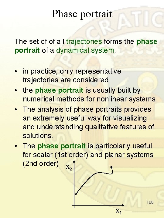
Phase portrait The set of of all trajectories forms the phase portrait of a dynamical system. • in practice, only representative trajectories are considered • the phase portrait is usually built by numerical methods for nonlinear systems • The analysis of phase portraits provides an extremely useful way for visualizing and understanding qualitative features of solutions. • The phase portrait is particolarly useful for scalar (1 st order) and planar systems (2 nd order) x 2 106 x 1

Transients and regimes • The orbits may have a bounded or unbounded asymptotic behavior (for t ± ). • If an orbit has a bounded asymptotic behavior for t + , the part of the orbit describing such an asymptotic behavior is referred to as regime and the remaining part is referred to as transient. • The simplest and most well known regime (bounded) is the equilibrium point (steady-state point), which is possible for every system order n 107

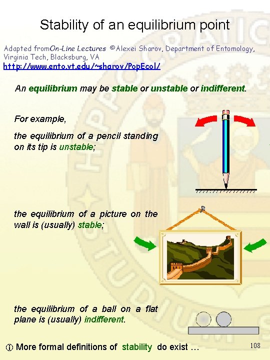
Stability of an equilibrium point Adapted from. On-Line Lectures ©Alexei Sharov, Department of Entomology, Virginia Tech, Blacksburg, VA http: //www. ento. vt. edu/~sharov/Pop. Ecol/ An equilibrium may be stable or unstable or indifferent. For example, the equilibrium of a pencil standing on its tip is unstable; the equilibrium of a picture on the wall is (usually) stable; the equilibrium of a ball on a flat plane is (usually) indifferent. More formal definitions of stability do exist … 108

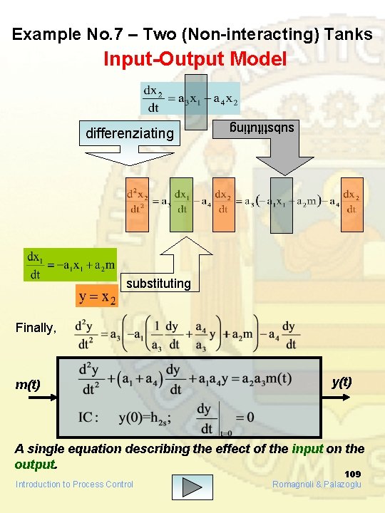
Example No. 7 – Two (Non-interacting) Tanks Input-Output Model substituting differenziating substituting Finally, m(t) y(t) A single equation describing the effect of the input on the output. Introduction to Process Control 109 Romagnoli & Palazoglu

Mathematical Models 4 th classification (based on the type of description adopted for time as the independent variable) VALID for DYNAMICAL SYSTEMS only 1. continuous time models 2. discrete time models 110

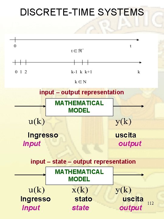
CONTINUOUS-TIME SYSTEMS The time changes continuously. It is not possible to define a minimum time interval: it is always possible to consider a smaller time interval. Accordingly, theory of continuoustime systems has been defined and studied, where the variables of the system are continuous-time functions, that is, at every time instant t, it is possible to define and assign the variable value. Continuous-time systems: t ℜ 111

DISCRETE-TIME SYSTEMS input – output representation MATHEMATICAL MODEL Ingresso Input uscita output input – state – output representation MATHEMATICAL MODEL Ingresso Input stato state uscita output 112

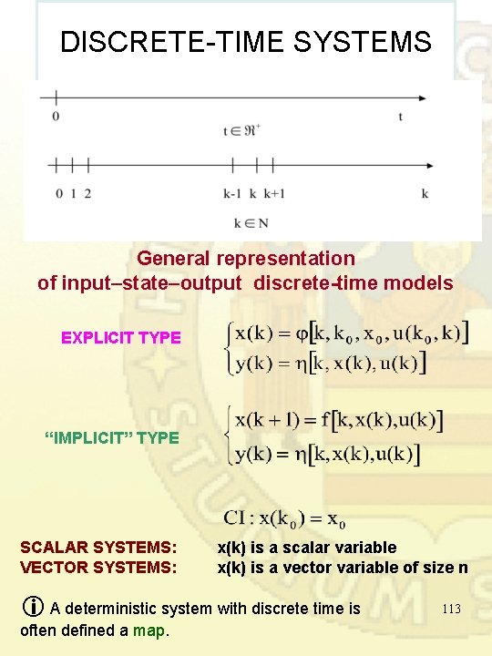
DISCRETE-TIME SYSTEMS General representation of input–state–output discrete-time models EXPLICIT TYPE “IMPLICIT” TYPE SCALAR SYSTEMS: VECTOR SYSTEMS: x(k) is a scalar variable x(k) is a vector variable of size n A deterministic system with discrete time is often defined a map. 113

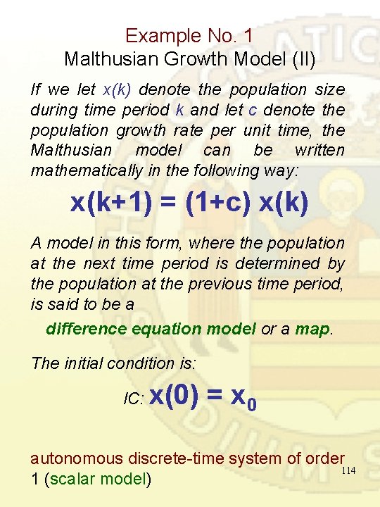
Example No. 1 Malthusian Growth Model (II) If we let x(k) denote the population size during time period k and let c denote the population growth rate per unit time, the Malthusian model can be written mathematically in the following way: x(k+1) = (1+c) x(k) A model in this form, where the population at the next time period is determined by the population at the previous time period, is said to be a difference equation model or a map. The initial condition is: IC: x(0) = x 0 autonomous discrete-time system of order 114 1 (scalar model)

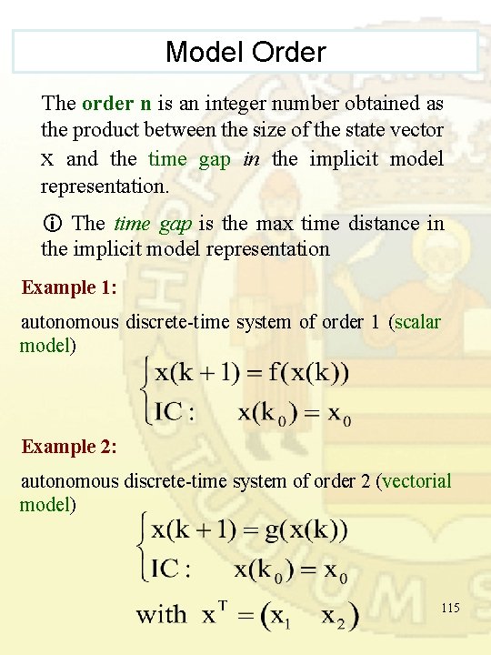
Model Order The order n is an integer number obtained as the product between the size of the state vector x and the time gap in the implicit model representation. The time gap is the max time distance in the implicit model representation Example 1: autonomous discrete-time system of order 1 (scalar model) Example 2: autonomous discrete-time system of order 2 (vectorial model) 115

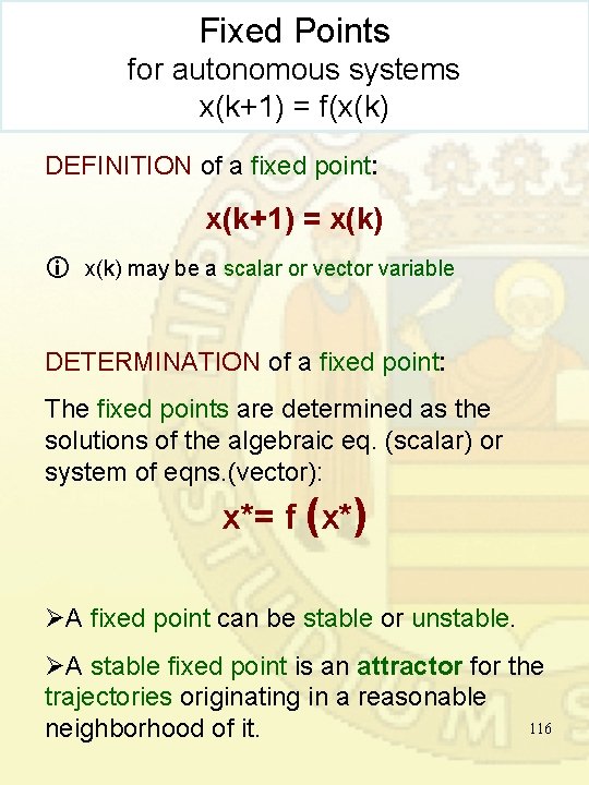
Fixed Points for autonomous systems x(k+1) = f(x(k) DEFINITION of a fixed point: x(k+1) = x(k) may be a scalar or vector variable DETERMINATION of a fixed point: The fixed points are determined as the solutions of the algebraic eq. (scalar) or system of eqns. (vector): x*= f (x*) ØA fixed point can be stable or unstable. ØA stable fixed point is an attractor for the trajectories originating in a reasonable 116 neighborhood of it.

Orbits or Trajectories Example: autonomous non-linear, discrete-time model of order 2 fixed point initial condition 117

Example No. 2 Logistic Model Differently from the Malthusian model … • developed by Belgian mathematician Pierre Verhulst (1838) HYPOTHESES • resources are limited for growth: N(t)≤Nsat CLOSED-FORM SOLUTION Nsat N 0≠ 0 118

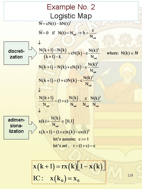
Example No. 2 Logistic Map discretization adimensionalization 119

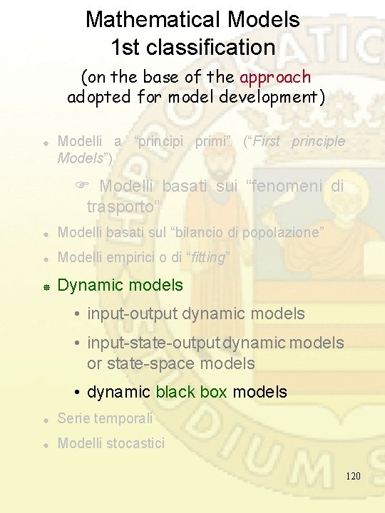
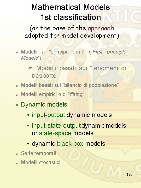
Mathematical Models 1 st classification (on the base of the approach adopted for model development) ] Modelli a “principi primi” (“First principle Models”) Modelli basati sui “fenomeni di trasporto” ] Modelli basati sul “bilancio di popolazione” ] Modelli empirici o di “fitting” ] Dynamic models • input-output dynamic models • input-state-output dynamic models or state-space models • dynamic black box models ] Serie temporali ] Modelli stocastici 120

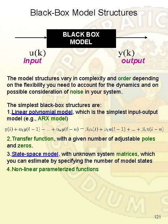
Black-Box Model Structures BLACK BOX MODEL Input output The model structures vary in complexity and order depending on the flexibility you need to account for the dynamics and on possible consideration of noise in your system. The simplest black-box structures are: 1. Linear polynomial model, which is the simplest input-output model (e. g. , ARX model) 2. Transfer function, with a given number of adjustable poles and zeros. 3. State-space model, with unknown system matrices, which you can estimate by specifying the number of model states 4. Non-linear parameterized functions 121

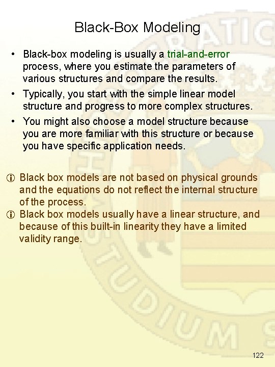
Black-Box Modeling • Black-box modeling is usually a trial-and-error process, where you estimate the parameters of various structures and compare the results. • Typically, you start with the simple linear model structure and progress to more complex structures. • You might also choose a model structure because you are more familiar with this structure or because you have specific application needs. Black box models are not based on physical grounds and the equations do not reflect the internal structure of the process. Black box models usually have a linear structure, and because of this built-in linearity they have a limited validity range. 122

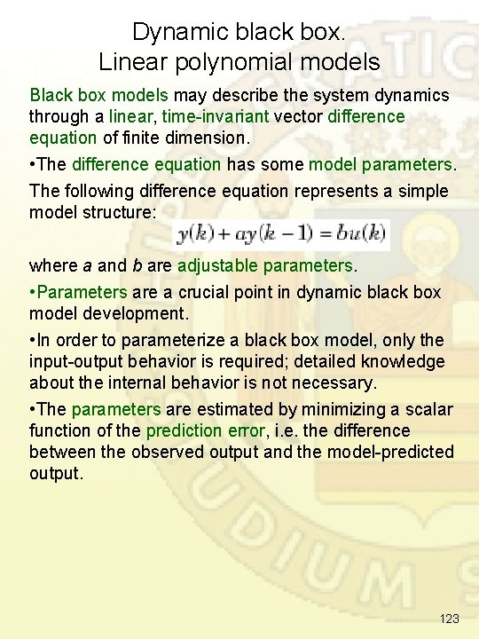
Dynamic black box. Linear polynomial models Black box models may describe the system dynamics through a linear, time-invariant vector difference equation of finite dimension. • The difference equation has some model parameters. The following difference equation represents a simple model structure: where a and b are adjustable parameters. • Parameters are a crucial point in dynamic black box model development. • In order to parameterize a black box model, only the input-output behavior is required; detailed knowledge about the internal behavior is not necessary. • The parameters are estimated by minimizing a scalar function of the prediction error, i. e. the difference between the observed output and the model-predicted output. 123

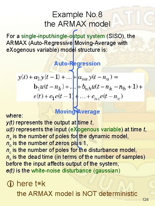
Example No. 8 the ARMAX model For a single-input/single-output system (SISO), the ARMAX (Auto-Regressive Moving-Average with e. Xogenous variable) model structure is: Auto-Regression Moving-Average where: y(t) represents the output at time t, u(t) represents the input (e. Xogenous variable) at time t, na is the number of poles for the dynamic model, nb is the number of zeros plus 1, nc is the number of poles for the disturbance model, nk is the dead time (in terms of the number of samples) before the input affects output of the system, e(t) is the white-noise disturbance (gaussian) here t≅k the ARMAX model is NOT deterministic 124

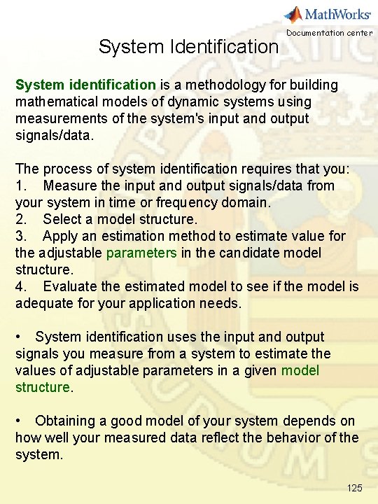
System Identification Documentation center System identification is a methodology for building mathematical models of dynamic systems using measurements of the system's input and output signals/data. The process of system identification requires that you: 1. Measure the input and output signals/data from your system in time or frequency domain. 2. Select a model structure. 3. Apply an estimation method to estimate value for the adjustable parameters in the candidate model structure. 4. Evaluate the estimated model to see if the model is adequate for your application needs. • System identification uses the input and output signals you measure from a system to estimate the values of adjustable parameters in a given model structure. • Obtaining a good model of your system depends on how well your measured data reflect the behavior of the system. 125

Mathematical Models 1 st classification (on the base of the approach adopted for model development) ] Modelli a “principi primi” (“First principle Models”) Modelli basati sui “fenomeni di trasporto” ] Modelli basati sul “bilancio di popolazione” ] Modelli empirici o di “fitting” ] Dynamic models • input-output dynamic models • input-state-output dynamic models or state-space models • dynamic black box models ] Serie temporali ] Modelli stocastici 126

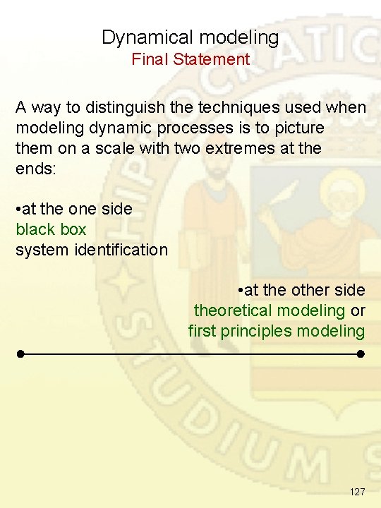
Dynamical modeling Final Statement A way to distinguish the techniques used when modeling dynamic processes is to picture them on a scale with two extremes at the ends: • at the one side black box system identification • at the other side theoretical modeling or first principles modeling 127

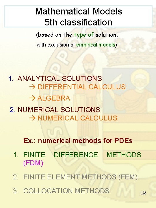
Mathematical Models 5 th classification (based on the type of solution, with exclusion of empirical models) 1. ANALYTICAL SOLUTIONS DIFFERENTIAL CALCULUS ALGEBRA 2. NUMERICAL SOLUTIONS NUMERICAL CALCULUS Ex. : numerical methods for PDEs 1. FINITE DIFFERENCE METHODS (FDM) 2. FINITE ELEMENT METHODS (FEM) 3. COLLOCATION METHODS 128

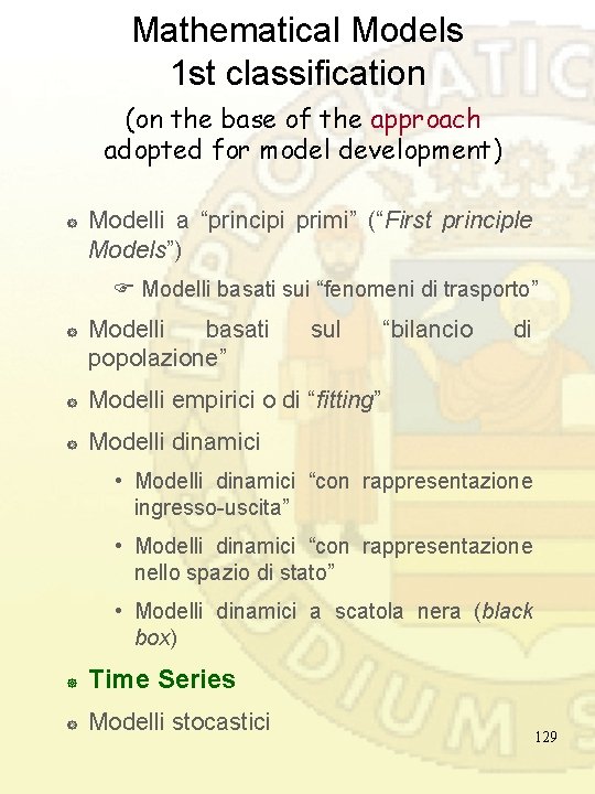
Mathematical Models 1 st classification (on the base of the approach adopted for model development) ] Modelli a “principi primi” (“First principle Models”) Modelli basati sui “fenomeni di trasporto” ] Modelli basati popolazione” sul ] Modelli empirici o di “fitting” ] Modelli dinamici “bilancio di • Modelli dinamici “con rappresentazione ingresso-uscita” • Modelli dinamici “con rappresentazione nello spazio di stato” • Modelli dinamici a scatola nera (black box) ] Time Series ] Modelli stocastici 129