FIL Epoch Eventrelated f MRI SPM Course 2002

FIL (Epoch &) Event-related f. MRI SPM Course 2002 Christian Buechel Karl Friston Rik Henson Oliver Josephs Wellcome Department of Cognitive Neurology & Institute of Cognitive Neuroscience University College London UK

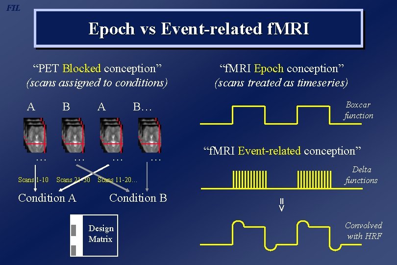
FIL Epoch vs Event-related f. MRI “PET Blocked conception” (scans assigned to conditions) A … Scans 1 -10 B A … … “f. MRI Event-related conception” Delta functions Scans 11 -20… Condition B Design Matrix => Condition A Boxcar function B… … Scans 21 -30 “f. MRI Epoch conception” (scans treated as timeseries) Convolved with HRF

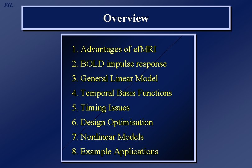
FIL Overview 1. Advantages of ef. MRI 2. BOLD impulse response 3. General Linear Model 4. Temporal Basis Functions 5. Timing Issues 6. Design Optimisation 7. Nonlinear Models 8. Example Applications

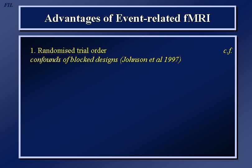
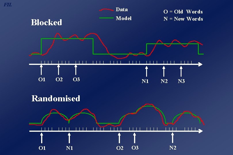
FIL Advantages of Event-related f. MRI 1. Randomised trial order confounds of blocked designs (Johnson et al 1997) c. f.

FIL Data Model Blocked O 1 O 2 O = Old Words N = New Words O 3 N 1 N 2 N 3 Randomised O 1 N 1 O 2 O 3 N 2

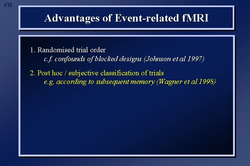
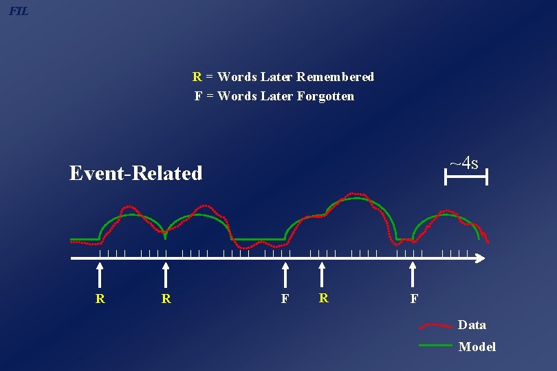
FIL Advantages of Event-related f. MRI 1. Randomised trial order c. f. confounds of blocked designs (Johnson et al 1997) 2. Post hoc / subjective classification of trials e. g, according to subsequent memory (Wagner et al 1998)

FIL R = Words Later Remembered F = Words Later Forgotten ~4 s Event-Related R R F Data Model

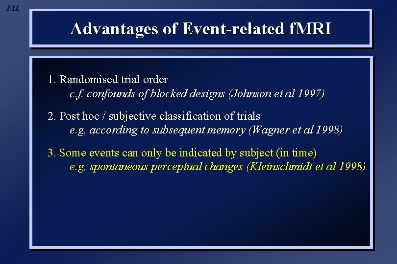
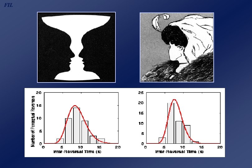
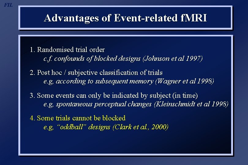
FIL Advantages of Event-related f. MRI 1. Randomised trial order c. f. confounds of blocked designs (Johnson et al 1997) 2. Post hoc / subjective classification of trials e. g, according to subsequent memory (Wagner et al 1998) 3. Some events can only be indicated by subject (in time) e. g, spontaneous perceptual changes (Kleinschmidt et al 1998)

FIL

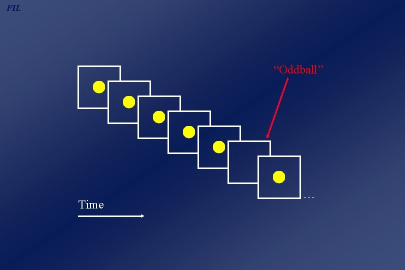
FIL Advantages of Event-related f. MRI 1. Randomised trial order c. f. confounds of blocked designs (Johnson et al 1997) 2. Post hoc / subjective classification of trials e. g, according to subsequent memory (Wagner et al 1998) 3. Some events can only be indicated by subject (in time) e. g, spontaneous perceptual changes (Kleinschmidt et al 1998) 4. Some trials cannot be blocked e. g, “oddball” designs (Clark et al. , 2000)

FIL “Oddball” Time …

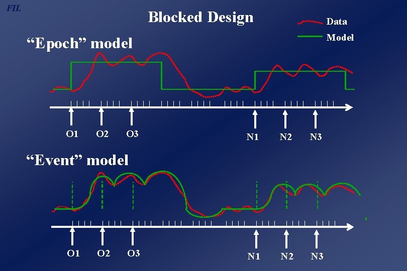
FIL Advantages of Event-related f. MRI 1. Randomised trial order c. f. confounds of blocked designs (Johnson et al 1997) 2. Post hoc / subjective classification of trials e. g, according to subsequent memory (Wagner et al 1998) 3. Some events can only be indicated by subject (in time) e. g, spontaneous perceptual changes (Kleinschmidt et al 1998) 4. Some trials cannot be blocked e. g, “oddball” designs (Clark et al. , 2000) 5. More accurate models even for blocked designs? e. g, “state-item” interactions (Chawla et al, 1999)

FIL Blocked Design Data Model “Epoch” model O 1 O 2 O 3 N 1 N 2 N 3 “Event” model O 1 O 2 O 3

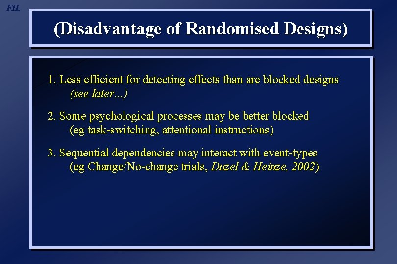
FIL (Disadvantage of Randomised Designs) 1. Less efficient for detecting effects than are blocked designs (see later…) 2. Some psychological processes may be better blocked (eg task-switching, attentional instructions) 3. Sequential dependencies may interact with event-types (eg Change/No-change trials, Duzel & Heinze, 2002)

FIL Overview 1. Advantages of ef. MRI 2. BOLD impulse response 3. General Linear Model 4. Temporal Basis Functions 5. Timing Issues 6. Design Optimisation 7. Nonlinear Models 8. Example Applications

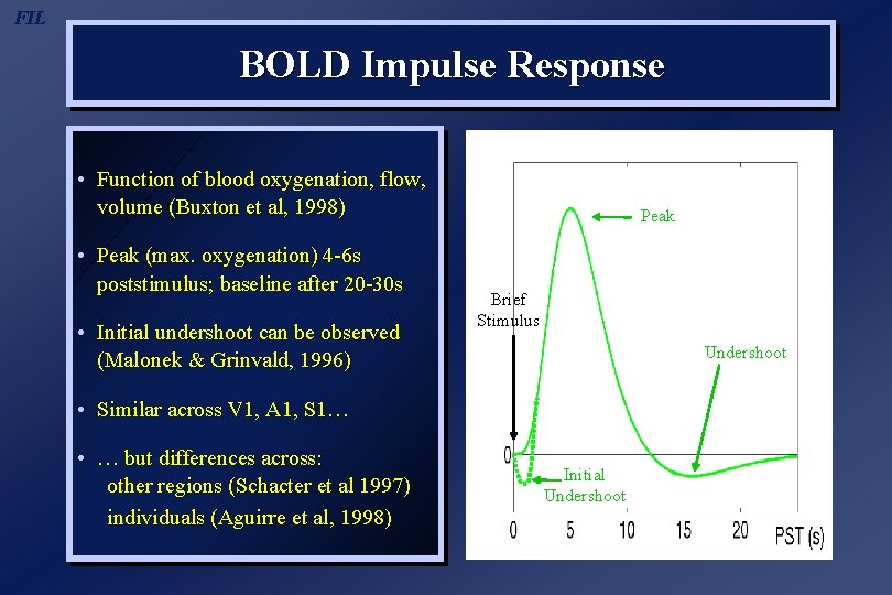
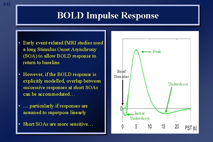
FIL BOLD Impulse Response • Function of blood oxygenation, flow, volume (Buxton et al, 1998) • Peak (max. oxygenation) 4 -6 s poststimulus; baseline after 20 -30 s • Initial undershoot can be observed (Malonek & Grinvald, 1996) Peak Brief Stimulus Undershoot • Similar across V 1, A 1, S 1… • … but differences across: other regions (Schacter et al 1997) individuals (Aguirre et al, 1998) Initial Undershoot

FIL BOLD Impulse Response • Early event-related f. MRI studies used a long Stimulus Onset Asynchrony (SOA) to allow BOLD response to return to baseline • However, if the BOLD response is explicitly modelled, overlap between successive responses at short SOAs can be accommodated… • … particularly if responses are assumed to superpose linearly • Short SOAs are more sensitive… Peak Brief Stimulus Undershoot Initial Undershoot

FIL Overview 1. Advantages of ef. MRI 2. BOLD impulse response 3. General Linear Model 4. Temporal Basis Functions 5. Timing Issues 6. Design Optimisation 7. Nonlinear Models 8. Example Applications

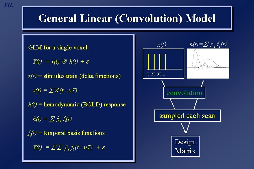
FIL General Linear (Convolution) Model GLM for a single voxel: x(t) h(t)= ßi fi (t) Y(t) = x(t) h(t) + x(t) = stimulus train (delta functions) x(t) = (t - n. T) T 2 T 3 T. . . convolution h(t) = hemodynamic (BOLD) response h(t) = ßi fi(t) sampled each scan fi(t) = temporal basis functions Y(t) = ßi fi (t - n. T) + Design Matrix

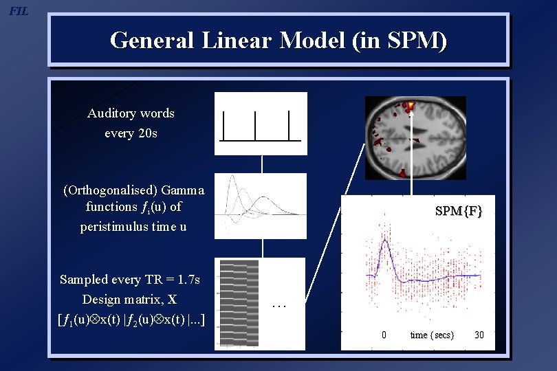
FIL General Linear Model (in SPM) Auditory words every 20 s (Orthogonalised) Gamma functions ƒi(u) of peristimulus time u Sampled every TR = 1. 7 s Design matrix, X [ƒ 1(u) x(t) |ƒ 2(u) x(t) |. . . ] SPM{F} … 0 time {secs} 30

FIL Overview 1. Advantages of ef. MRI 2. BOLD impulse response 3. General Linear Model 4. Temporal Basis Functions 5. Timing Issues 6. Design Optimisation 7. Nonlinear Models 8. Example Applications

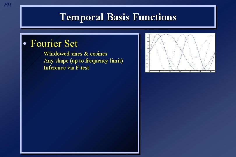
FIL Temporal Basis Functions • Fourier Set Windowed sines & cosines Any shape (up to frequency limit) Inference via F-test

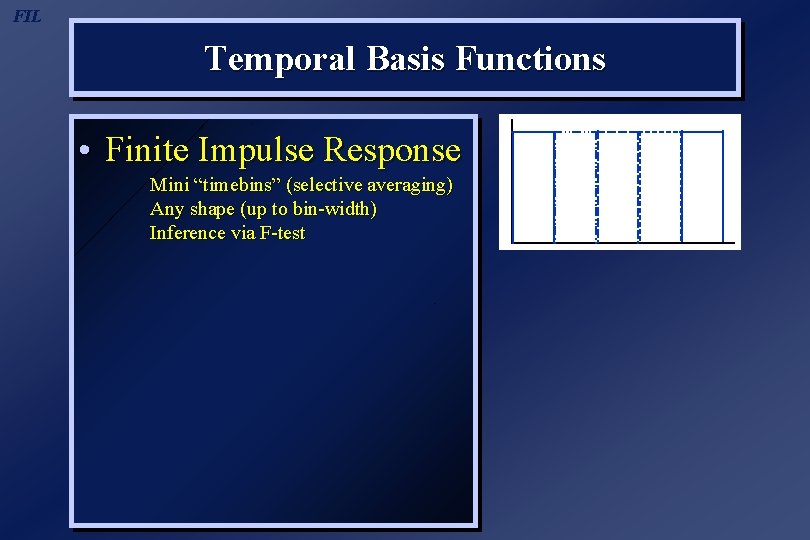
FIL Temporal Basis Functions • Finite Impulse Response Mini “timebins” (selective averaging) Any shape (up to bin-width) Inference via F-test

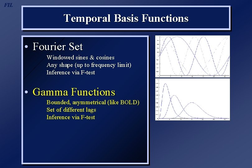
FIL Temporal Basis Functions • Fourier Set Windowed sines & cosines Any shape (up to frequency limit) Inference via F-test • Gamma Functions Bounded, asymmetrical (like BOLD) Set of different lags Inference via F-test

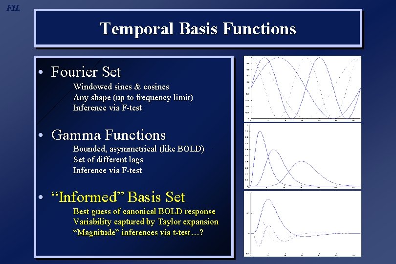
FIL Temporal Basis Functions • Fourier Set Windowed sines & cosines Any shape (up to frequency limit) Inference via F-test • Gamma Functions Bounded, asymmetrical (like BOLD) Set of different lags Inference via F-test • “Informed” Basis Set Best guess of canonical BOLD response Variability captured by Taylor expansion “Magnitude” inferences via t-test…?

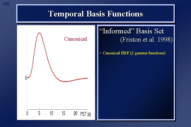
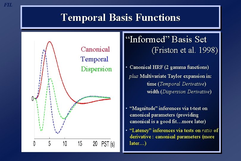
FIL Temporal Basis Functions “Informed” Basis Set Canonical (Friston et al. 1998) • Canonical HRF (2 gamma functions)

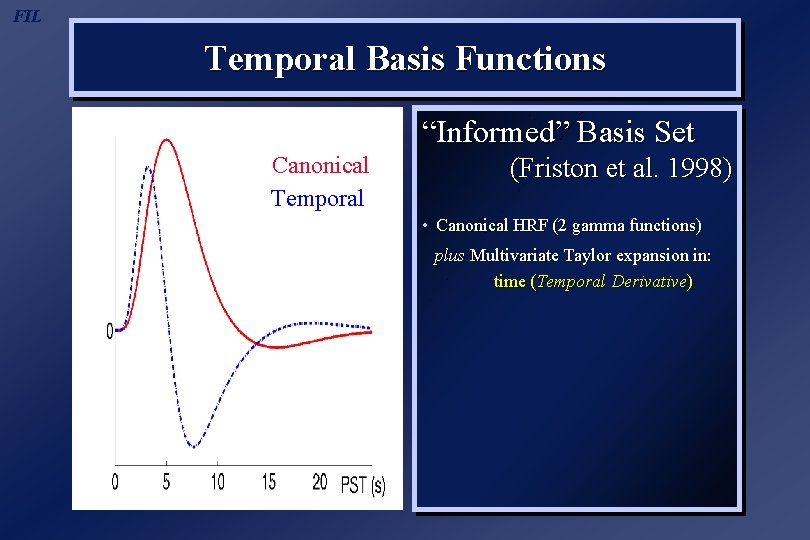
FIL Temporal Basis Functions “Informed” Basis Set Canonical Temporal (Friston et al. 1998) • Canonical HRF (2 gamma functions) plus Multivariate Taylor expansion in: time (Temporal Derivative)

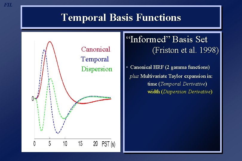
FIL Temporal Basis Functions “Informed” Basis Set Canonical Temporal Dispersion (Friston et al. 1998) • Canonical HRF (2 gamma functions) plus Multivariate Taylor expansion in: time (Temporal Derivative) width (Dispersion Derivative)

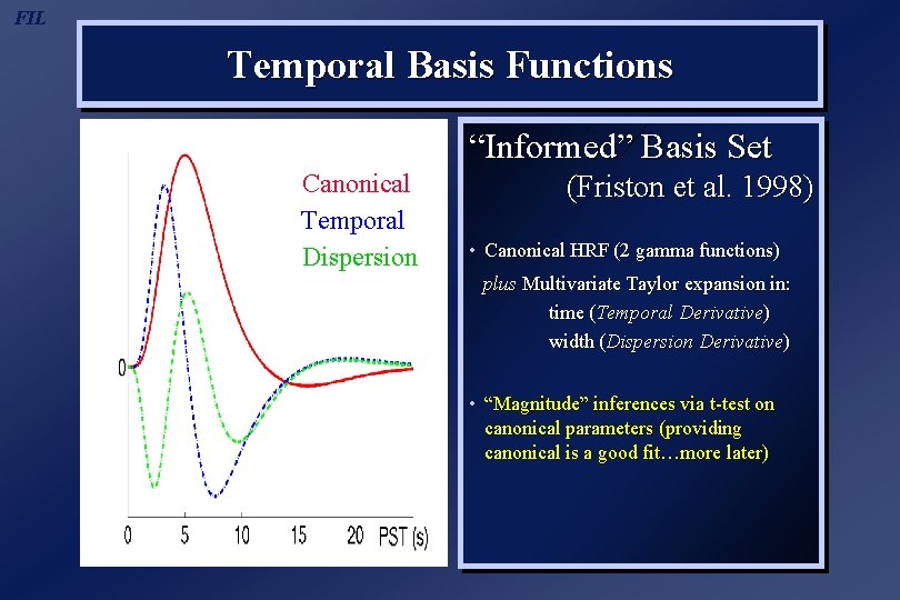
FIL Temporal Basis Functions “Informed” Basis Set Canonical Temporal Dispersion (Friston et al. 1998) • Canonical HRF (2 gamma functions) plus Multivariate Taylor expansion in: time (Temporal Derivative) width (Dispersion Derivative) • “Magnitude” inferences via t-test on canonical parameters (providing canonical is a good fit…more later)

FIL Temporal Basis Functions “Informed” Basis Set Canonical Temporal Dispersion (Friston et al. 1998) • Canonical HRF (2 gamma functions) plus Multivariate Taylor expansion in: time (Temporal Derivative) width (Dispersion Derivative) • “Magnitude” inferences via t-test on canonical parameters (providing canonical is a good fit…more later) • “Latency” inferences via tests on ratio of derivative : canonical parameters (more later…)

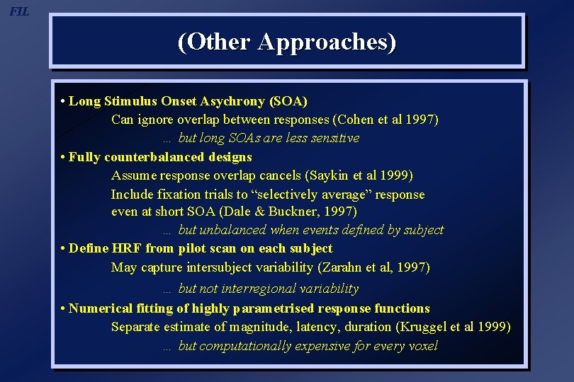
FIL (Other Approaches) • Long Stimulus Onset Asychrony (SOA) Can ignore overlap between responses (Cohen et al 1997) … but long SOAs are less sensitive • Fully counterbalanced designs Assume response overlap cancels (Saykin et al 1999) Include fixation trials to “selectively average” response even at short SOA (Dale & Buckner, 1997) … but unbalanced when events defined by subject • Define HRF from pilot scan on each subject May capture intersubject variability (Zarahn et al, 1997) … but not interregional variability • Numerical fitting of highly parametrised response functions Separate estimate of magnitude, latency, duration (Kruggel et al 1999) … but computationally expensive for every voxel

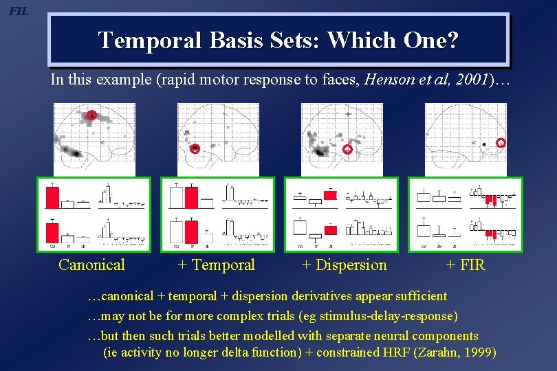
FIL Temporal Basis Sets: Which One? In this example (rapid motor response to faces, Henson et al, 2001)… Canonical + Temporal + Dispersion + FIR …canonical + temporal + dispersion derivatives appear sufficient …may not be for more complex trials (eg stimulus-delay-response) …but then such trials better modelled with separate neural components (ie activity no longer delta function) + constrained HRF (Zarahn, 1999)

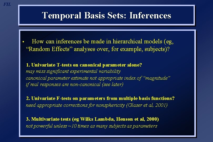
FIL Temporal Basis Sets: Inferences • How can inferences be made in hierarchical models (eg, “Random Effects” analyses over, for example, subjects)? 1. Univariate T-tests on canonical parameter alone? may miss significant experimental variability canonical parameter estimate not appropriate index of “magnitude” if real responses are non-canonical (see later) 2. Univariate F-tests on parameters from multiple basis functions? need appropriate corrections for nonsphericity (Glaser et al, 2001) 3. Multivariate tests (eg Wilks Lambda, Henson et al, 2000) not powerful unless ~10 times as many subjects as parameters

FIL Overview 1. Advantages of ef. MRI 2. BOLD impulse response 3. General Linear Model 4. Temporal Basis Functions 5. Timing Issues 6. Design Optimisation 7. Nonlinear Models 8. Example Applications

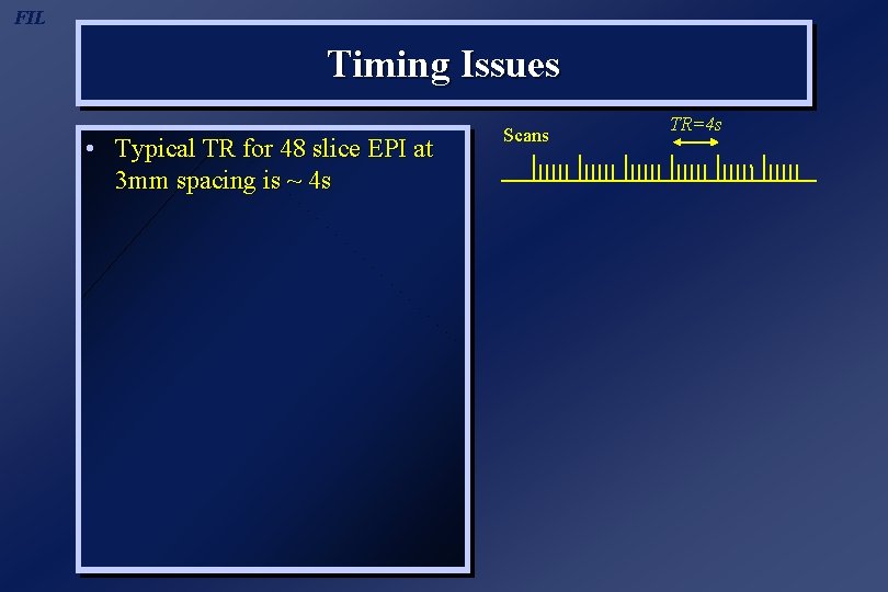
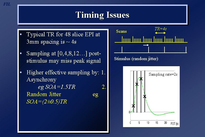
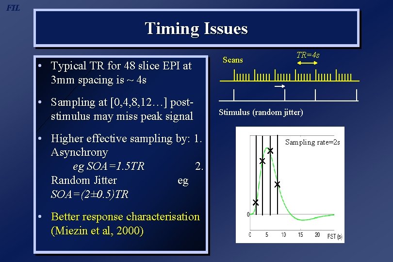
FIL Timing Issues • Typical TR for 48 slice EPI at 3 mm spacing is ~ 4 s Scans TR=4 s

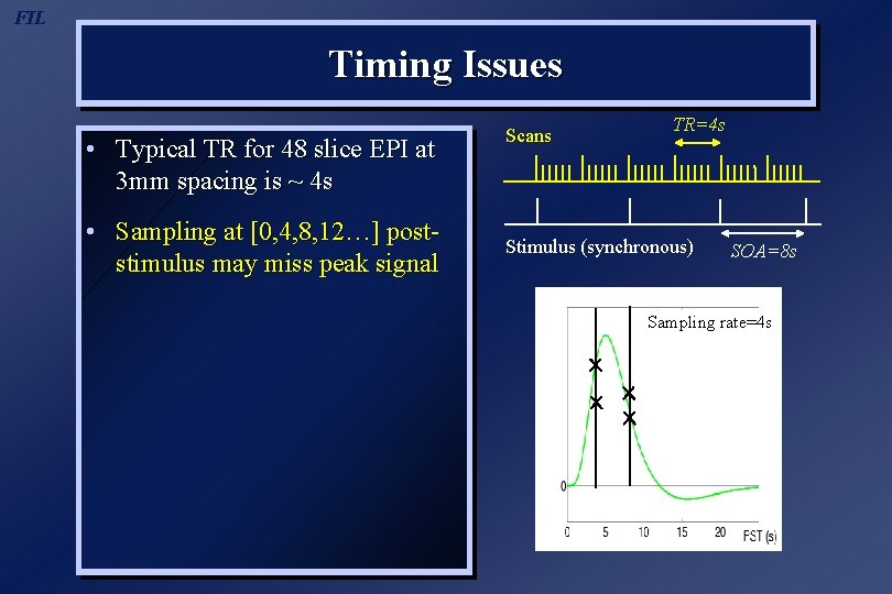
FIL Timing Issues • Typical TR for 48 slice EPI at 3 mm spacing is ~ 4 s • Sampling at [0, 4, 8, 12…] poststimulus may miss peak signal Scans TR=4 s Stimulus (synchronous) SOA=8 s Sampling rate=4 s

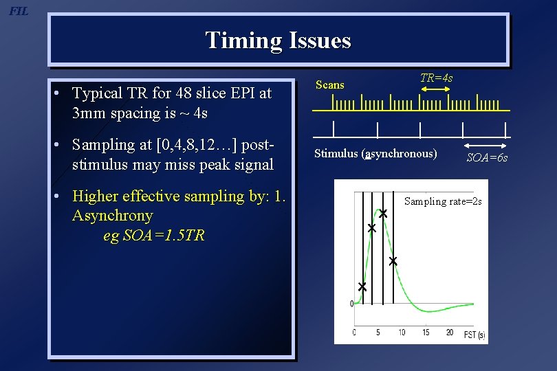
FIL Timing Issues • Typical TR for 48 slice EPI at 3 mm spacing is ~ 4 s • Sampling at [0, 4, 8, 12…] poststimulus may miss peak signal • Higher effective sampling by: 1. Asynchrony eg SOA=1. 5 TR Scans TR=4 s Stimulus (asynchronous) SOA=6 s Sampling rate=2 s

FIL Timing Issues • Typical TR for 48 slice EPI at 3 mm spacing is ~ 4 s • Sampling at [0, 4, 8, 12…] poststimulus may miss peak signal • Higher effective sampling by: 1. Asynchrony eg SOA=1. 5 TR 2. Random Jitter eg SOA=(2± 0. 5)TR Scans TR=4 s Stimulus (random jitter) Sampling rate=2 s

FIL Timing Issues • Typical TR for 48 slice EPI at 3 mm spacing is ~ 4 s • Sampling at [0, 4, 8, 12…] poststimulus may miss peak signal • Higher effective sampling by: 1. Asynchrony eg SOA=1. 5 TR 2. Random Jitter eg SOA=(2± 0. 5)TR • Better response characterisation (Miezin et al, 2000) Scans TR=4 s Stimulus (random jitter) Sampling rate=2 s

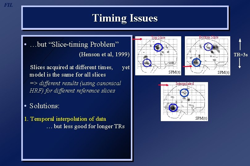
FIL Timing Issues • …but “Slice-timing Problem” (Henson et al, 1999) Slices acquired at different times, model is the same for all slices yet

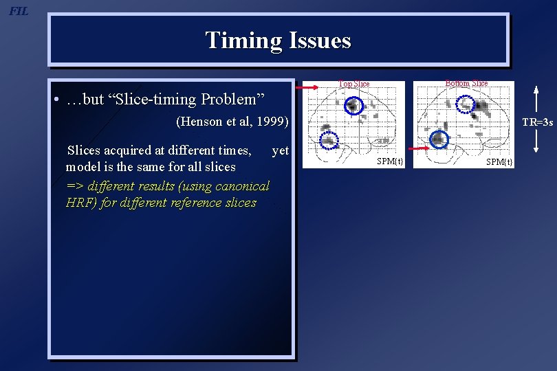
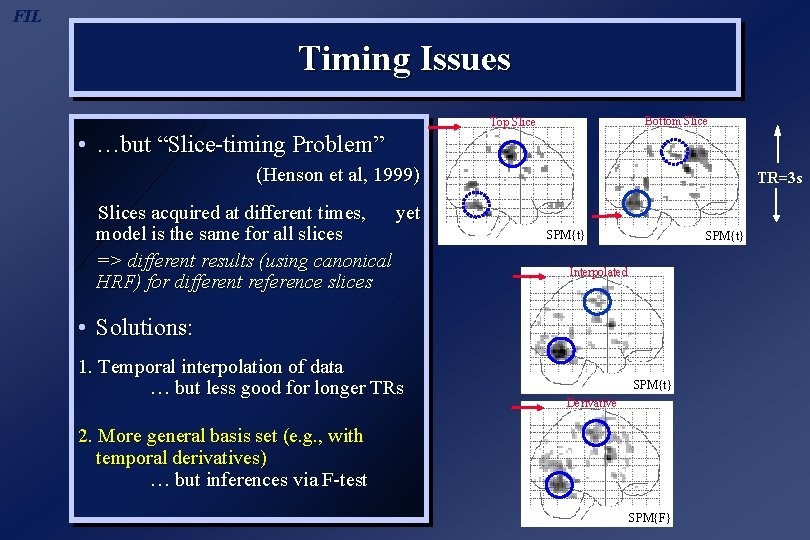
FIL Timing Issues Bottom Slice Top Slice • …but “Slice-timing Problem” (Henson et al, 1999) Slices acquired at different times, yet model is the same for all slices => different results (using canonical HRF) for different reference slices TR=3 s SPM{t}

FIL Timing Issues Bottom Slice Top Slice • …but “Slice-timing Problem” (Henson et al, 1999) Slices acquired at different times, yet model is the same for all slices => different results (using canonical HRF) for different reference slices TR=3 s SPM{t} Interpolated • Solutions: 1. Temporal interpolation of data … but less good for longer TRs SPM{t}

FIL Timing Issues Bottom Slice Top Slice • …but “Slice-timing Problem” (Henson et al, 1999) Slices acquired at different times, yet model is the same for all slices => different results (using canonical HRF) for different reference slices TR=3 s SPM{t} Interpolated • Solutions: 1. Temporal interpolation of data … but less good for longer TRs SPM{t} Derivative 2. More general basis set (e. g. , with temporal derivatives) … but inferences via F-test SPM{F}

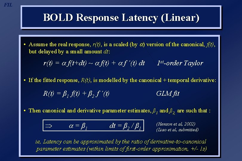
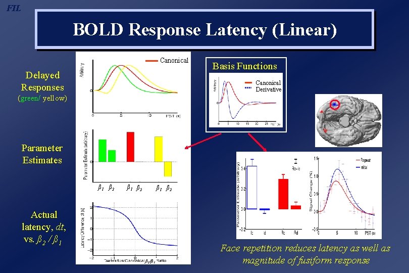
FIL BOLD Response Latency (Linear) • Assume the real response, r(t), is a scaled (by ) version of the canonical, f(t), but delayed by a small amount dt: r(t) = f(t+dt) ~ f(t) + f ´(t) dt 1 st-order Taylor • If the fitted response, R(t), is modelled by the canonical + temporal derivative: R(t) = ß 1 f(t) + ß 2 f ´(t) GLM fit • Then canonical and derivative parameter estimates, ß 1 and ß 2, are such that : Þ = ß 1 dt = ß 2 / ß 1 (Henson et al, 2002) (Liao et al, submitted) ie, Latency can be approximated by the ratio of derivative-to-canonical parameter estimates (within limits of first-order approximation, +/- 1 s)

FIL BOLD Response Latency (Linear) Canonical Delayed Responses Basis Functions Canonical Derivative (green/ yellow) Parameter Estimates ß 1 ß 2 Actual latency, dt, vs. ß 2 / ß 1 ß 2 /ß 1 Face repetition reduces latency as well as magnitude of fusiform response

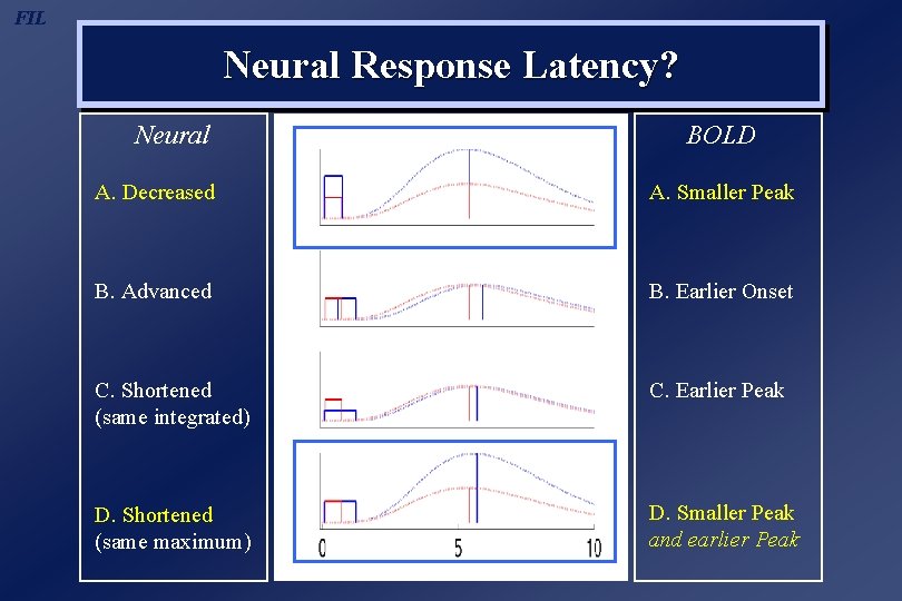
FIL Neural Response Latency? Neural BOLD A. Decreased A. Smaller Peak B. Advanced B. Earlier Onset C. Shortened (same integrated) C. Earlier Peak D. Shortened (same maximum) D. Smaller Peak and earlier Peak

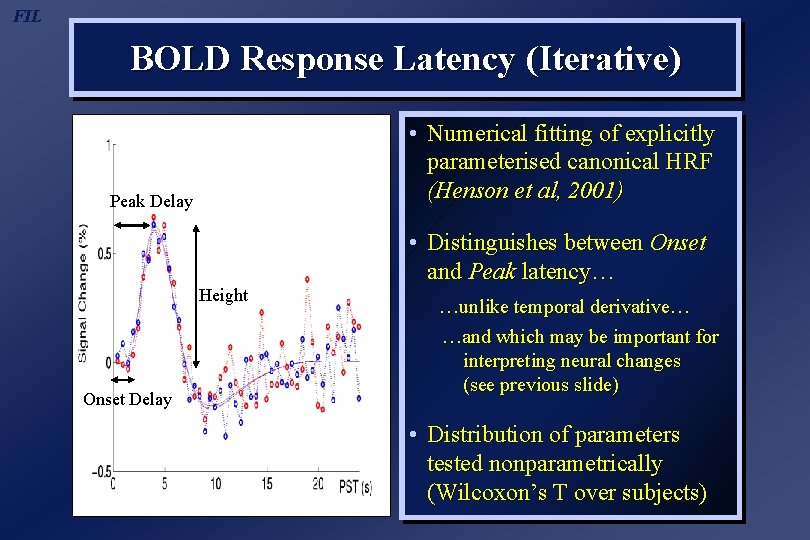
FIL BOLD Response Latency (Iterative) • Numerical fitting of explicitly parameterised canonical HRF (Henson et al, 2001) Peak Delay • Distinguishes between Onset and Peak latency… Height Onset Delay …unlike temporal derivative… …and which may be important for interpreting neural changes (see previous slide) • Distribution of parameters tested nonparametrically (Wilcoxon’s T over subjects)

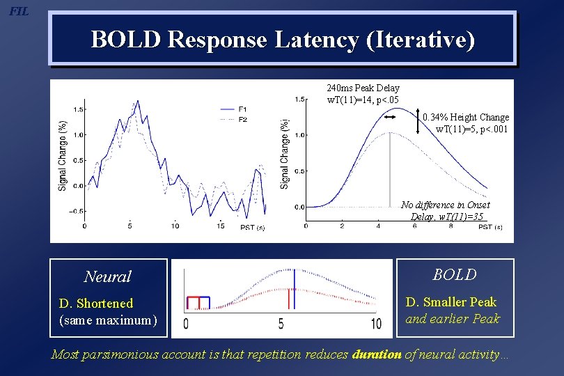
FIL BOLD Response Latency (Iterative) 240 ms Peak Delay w. T(11)=14, p<. 05 0. 34% Height Change w. T(11)=5, p<. 001 No difference in Onset Delay, w. T(11)=35 Neural BOLD D. Shortened (same maximum) D. Smaller Peak and earlier Peak Most parsimonious account is that repetition reduces duration of neural activity…

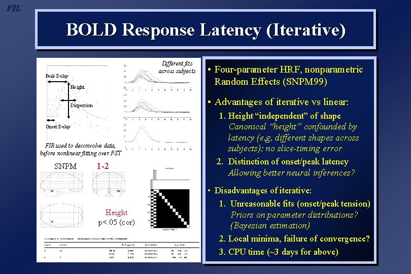
FIL BOLD Response Latency (Iterative) Different fits across subjects Peak Delay Height • Advantages of iterative vs linear: Dispersion Onset Delay FIR used to deconvolve data, before nonlinear fitting over PST SNPM • Four-parameter HRF, nonparametric Random Effects (SNPM 99) 1 -2 Height p<. 05 (cor) 1. Height “independent” of shape Canonical “height” confounded by latency (e. g, different shapes across subjects); no slice-timing error 2. Distinction of onset/peak latency Allowing better neural inferences? • Disadvantages of iterative: 1. Unreasonable fits (onset/peak tension) Priors on parameter distributions? (Bayesian estimation) 2. Local minima, failure of convergence? 3. CPU time (~3 days for above)

FIL Overview 1. Advantages of ef. MRI 2. BOLD impulse response 3. General Linear Model 4. Temporal Basis Functions 5. Timing Issues 6. Design Optimisation 7. Nonlinear Models 8. Example Applications

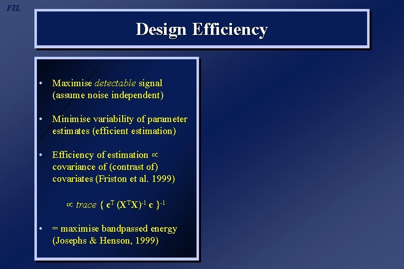
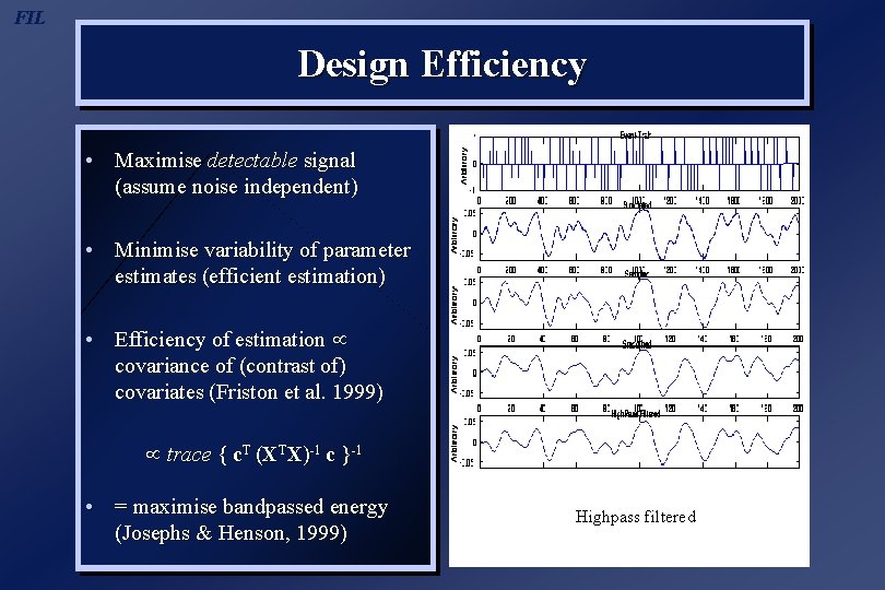
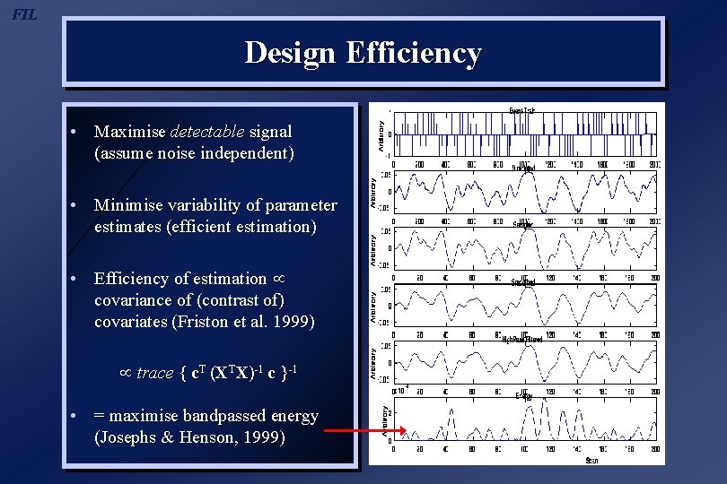
FIL Design Efficiency • Maximise detectable signal (assume noise independent) • Minimise variability of parameter estimates (efficient estimation) • Efficiency of estimation covariance of (contrast of) covariates (Friston et al. 1999) trace { c. T (XTX)-1 c }-1 • = maximise bandpassed energy (Josephs & Henson, 1999)

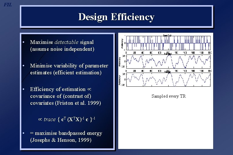
FIL Design Efficiency • Maximise detectable signal (assume noise independent) • Minimise variability of parameter estimates (efficient estimation) • Efficiency of estimation covariance of (contrast of) covariates (Friston et al. 1999) trace { c. T (XTX)-1 c }-1 • = maximise bandpassed energy (Josephs & Henson, 1999) Events (A-B)

FIL Design Efficiency • Maximise detectable signal (assume noise independent) • Minimise variability of parameter estimates (efficient estimation) • Efficiency of estimation covariance of (contrast of) covariates (Friston et al. 1999) trace { c. T (XTX)-1 c }-1 • = maximise bandpassed energy (Josephs & Henson, 1999) Convolved with HRF

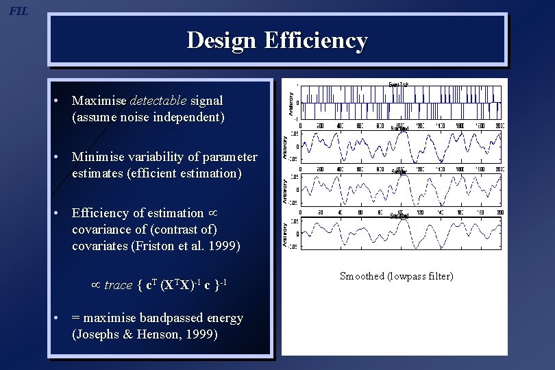
FIL Design Efficiency • Maximise detectable signal (assume noise independent) • Minimise variability of parameter estimates (efficient estimation) • Efficiency of estimation covariance of (contrast of) covariates (Friston et al. 1999) trace { c. T (XTX)-1 c }-1 • = maximise bandpassed energy (Josephs & Henson, 1999) Sampled every TR

FIL Design Efficiency • Maximise detectable signal (assume noise independent) • Minimise variability of parameter estimates (efficient estimation) • Efficiency of estimation covariance of (contrast of) covariates (Friston et al. 1999) trace { c. T (XTX)-1 c }-1 • = maximise bandpassed energy (Josephs & Henson, 1999) Smoothed (lowpass filter)

FIL Design Efficiency • Maximise detectable signal (assume noise independent) • Minimise variability of parameter estimates (efficient estimation) • Efficiency of estimation covariance of (contrast of) covariates (Friston et al. 1999) trace { c. T (XTX)-1 c }-1 • = maximise bandpassed energy (Josephs & Henson, 1999) Highpass filtered

FIL Design Efficiency • Maximise detectable signal (assume noise independent) • Minimise variability of parameter estimates (efficient estimation) • Efficiency of estimation covariance of (contrast of) covariates (Friston et al. 1999) trace { c. T (XTX)-1 c }-1 • = maximise bandpassed energy (Josephs & Henson, 1999)

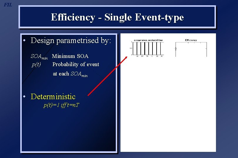
FIL Efficiency - Single Event-type • Design parametrised by: SOAmin Minimum SOA

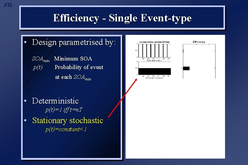
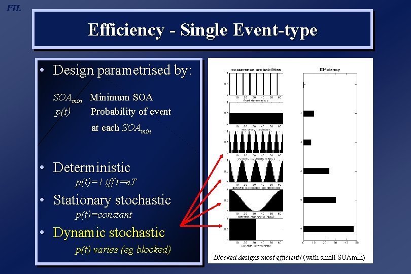
FIL Efficiency - Single Event-type • Design parametrised by: SOAmin Minimum SOA p(t) Probability of event at each SOAmin

FIL Efficiency - Single Event-type • Design parametrised by: SOAmin Minimum SOA p(t) Probability of event at each SOAmin • Deterministic p(t)=1 iff t=n. T

FIL Efficiency - Single Event-type • Design parametrised by: SOAmin Minimum SOA p(t) Probability of event at each SOAmin • Deterministic p(t)=1 iff t=n. T • Stationary stochastic p(t)=constant<1

FIL Efficiency - Single Event-type • Design parametrised by: SOAmin Minimum SOA p(t) Probability of event at each SOAmin • Deterministic p(t)=1 iff t=n. T • Stationary stochastic p(t)=constant • Dynamic stochastic p(t) varies (eg blocked) Blocked designs most efficient! (with small SOAmin)

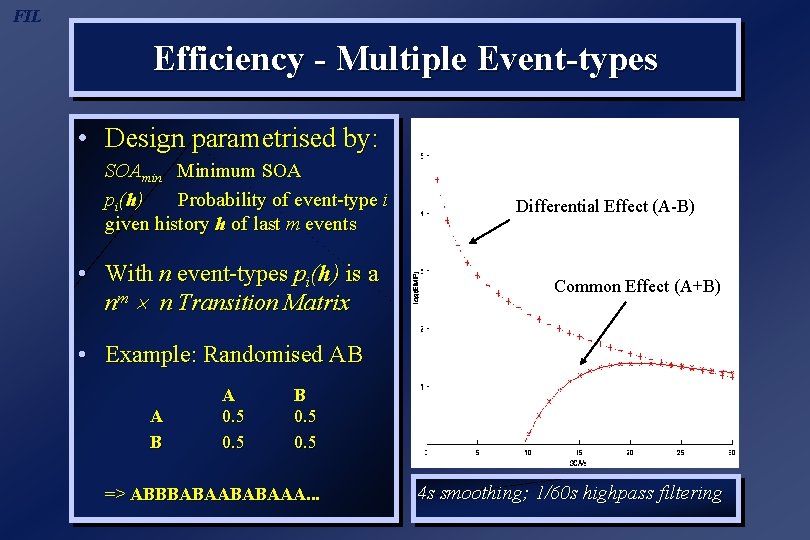
FIL Efficiency - Multiple Event-types • Design parametrised by: SOAmin Minimum SOA pi(h) Probability of event-type i given history h of last m events • With n event-types pi(h) is a nm n Transition Matrix Differential Effect (A-B) Common Effect (A+B) • Example: Randomised AB A 0. 5 B 0. 5 => ABBBABAAA. . . 4 s smoothing; 1/60 s highpass filtering

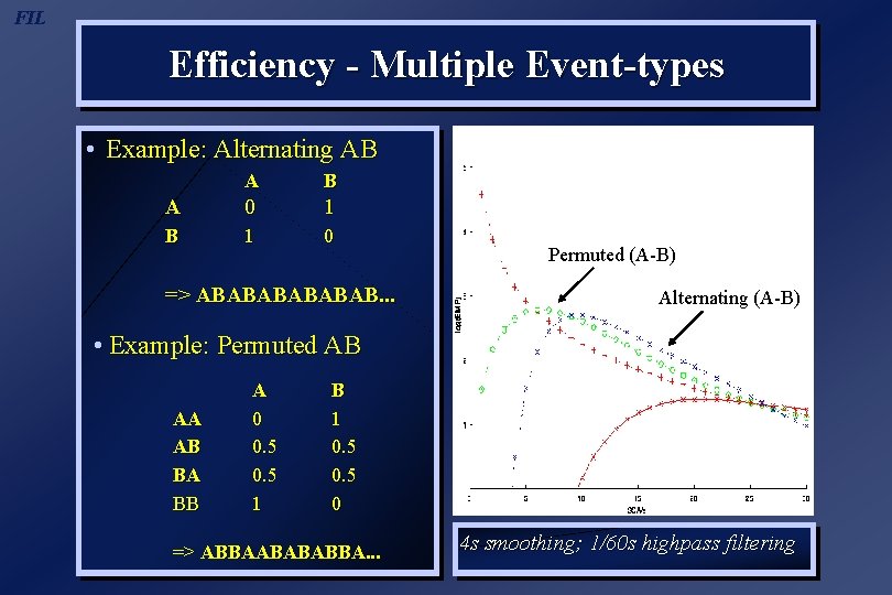
FIL Efficiency - Multiple Event-types • Example: Alternating AB A 0 1 B 1 0 => ABABAB. . . Permuted (A-B) Alternating (A-B) • Example: Permuted AB AA AB BA BB A 0 0. 5 1 B 1 0. 5 0 => ABBAABABABBA. . . 4 s smoothing; 1/60 s highpass filtering

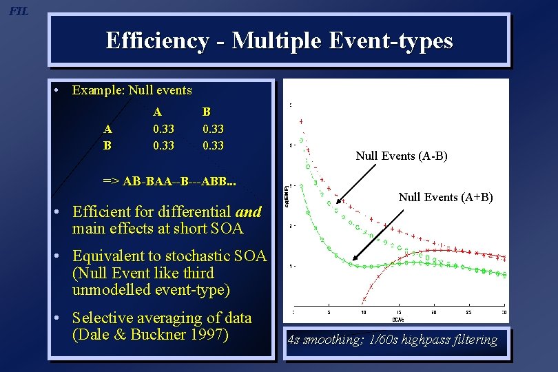
FIL Efficiency - Multiple Event-types • Example: Null events A B A 0. 33 B 0. 33 Null Events (A-B) => AB-BAA--B---ABB. . . • Efficient for differential and main effects at short SOA Null Events (A+B) • Equivalent to stochastic SOA (Null Event like third unmodelled event-type) • Selective averaging of data (Dale & Buckner 1997) 4 s smoothing; 1/60 s highpass filtering

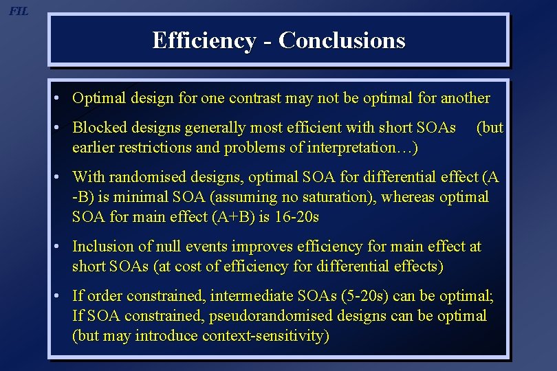
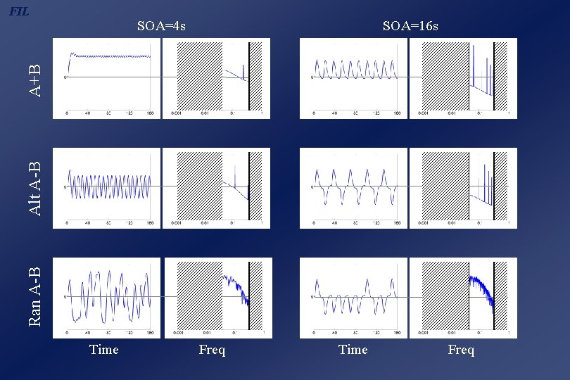
FIL Efficiency - Conclusions • Optimal design for one contrast may not be optimal for another • Blocked designs generally most efficient with short SOAs earlier restrictions and problems of interpretation…) (but • With randomised designs, optimal SOA for differential effect (A -B) is minimal SOA (assuming no saturation), whereas optimal SOA for main effect (A+B) is 16 -20 s • Inclusion of null events improves efficiency for main effect at short SOAs (at cost of efficiency for differential effects) • If order constrained, intermediate SOAs (5 -20 s) can be optimal; If SOA constrained, pseudorandomised designs can be optimal (but may introduce context-sensitivity)

FIL SOA=16 s Ran A-B Alt A-B A+B SOA=4 s Time Freq

FIL Overview 1. Advantages of ef. MRI 2. BOLD impulse response 3. General Linear Model 4. Temporal Basis Functions 5. Timing Issues 6. Design Optimisation 7. Nonlinear Models 8. Example Applications

FIL Nonlinear Model input u(t) [u(t)] response y(t) Stimulus function kernels (h) estimate Volterra series - a general nonlinear input-output model = 1[u(t)] + 2[u(t)] +. . + n[u(t)] +. . y(t) n[u(t)] = . . hn(t 1, . . . , tn)u(t - t 1). . u(t - tn)dt 1. . dtn

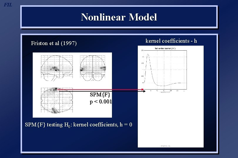
FIL Nonlinear Model kernel coefficients - h Friston et al (1997) SPM{F} p < 0. 001 SPM{F} testing H 0: kernel coefficients, h = 0

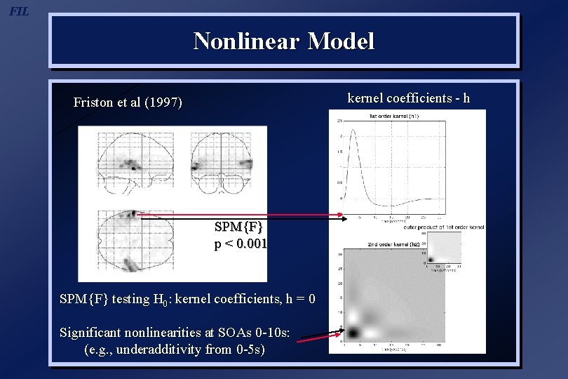
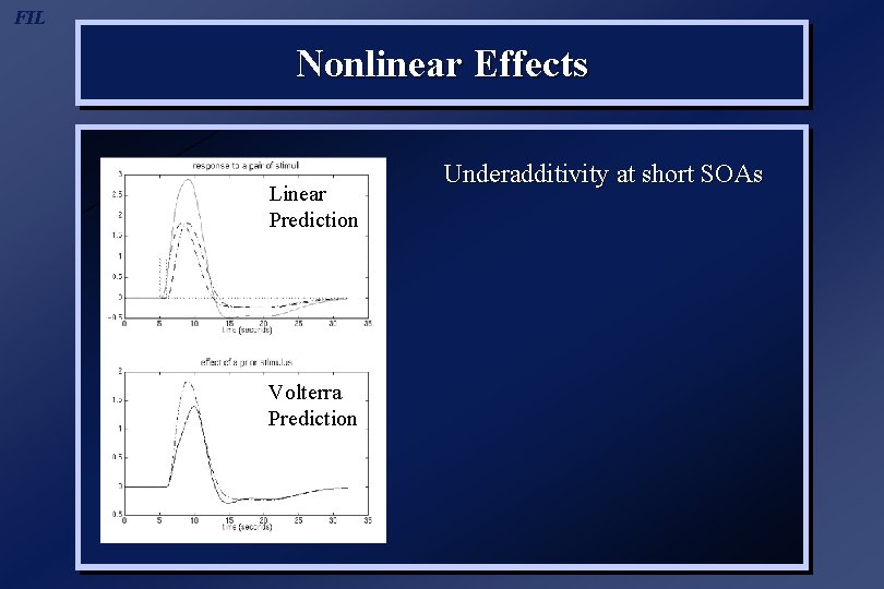
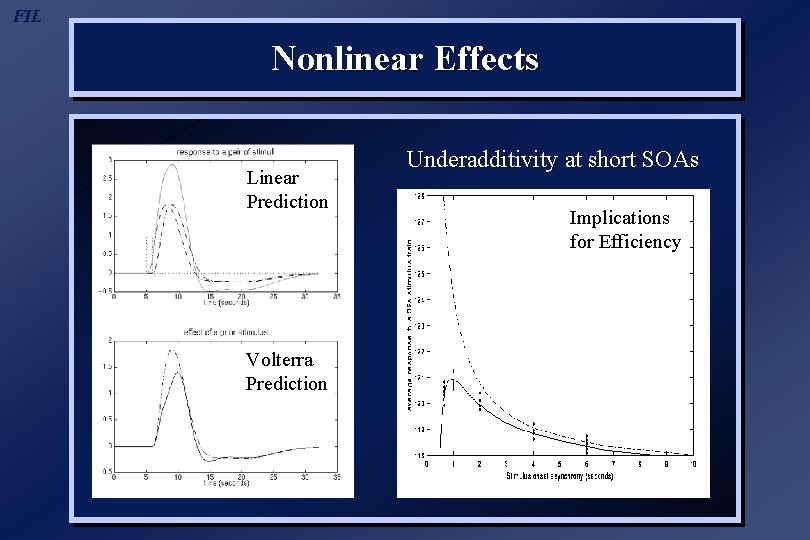
FIL Nonlinear Model kernel coefficients - h Friston et al (1997) SPM{F} p < 0. 001 SPM{F} testing H 0: kernel coefficients, h = 0 Significant nonlinearities at SOAs 0 -10 s: (e. g. , underadditivity from 0 -5 s)

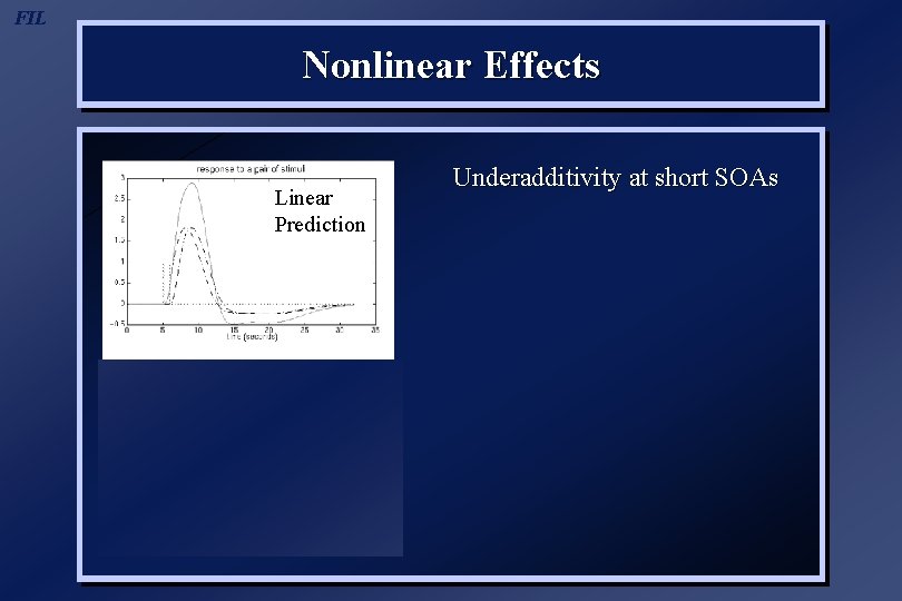
FIL Nonlinear Effects Linear Prediction Volterra Prediction Underadditivity at short SOAs

FIL Nonlinear Effects Linear Prediction Volterra Prediction Underadditivity at short SOAs

FIL Nonlinear Effects Linear Prediction Volterra Prediction Underadditivity at short SOAs Implications for Efficiency

FIL Overview 1. Advantages of ef. MRI 2. BOLD impulse response 3. General Linear Model 4. Temporal Basis Functions 5. Timing Issues 6. Design Optimisation 7. Nonlinear Models 8. Example Applications

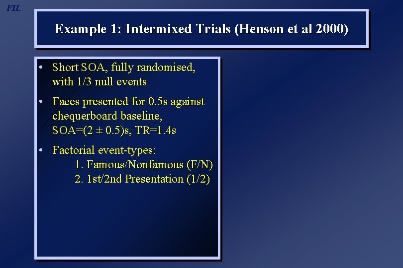
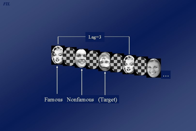
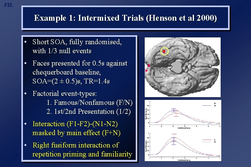
FIL Example 1: Intermixed Trials (Henson et al 2000) • Short SOA, fully randomised, with 1/3 null events • Faces presented for 0. 5 s against chequerboard baseline, SOA=(2 ± 0. 5)s, TR=1. 4 s • Factorial event-types: 1. Famous/Nonfamous (F/N) 2. 1 st/2 nd Presentation (1/2)

FIL Lag=3 . . . Famous Nonfamous (Target)

FIL Example 1: Intermixed Trials (Henson et al 2000) • Short SOA, fully randomised, with 1/3 null events • Faces presented for 0. 5 s against chequerboard baseline, SOA=(2 ± 0. 5)s, TR=1. 4 s • Factorial event-types: 1. Famous/Nonfamous (F/N) 2. 1 st/2 nd Presentation (1/2) • Interaction (F 1 -F 2)-(N 1 -N 2) masked by main effect (F+N) • Right fusiform interaction of repetition priming and familiarity

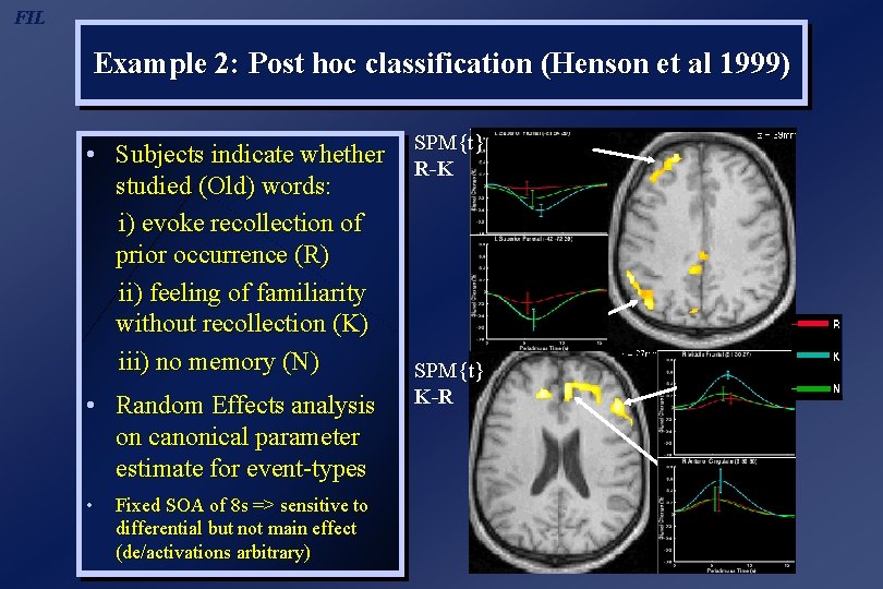
FIL Example 2: Post hoc classification (Henson et al 1999) • Subjects indicate whether studied (Old) words: i) evoke recollection of prior occurrence (R) ii) feeling of familiarity without recollection (K) iii) no memory (N) • Random Effects analysis on canonical parameter estimate for event-types • Fixed SOA of 8 s => sensitive to differential but not main effect (de/activations arbitrary) SPM{t} R-K SPM{t} K-R

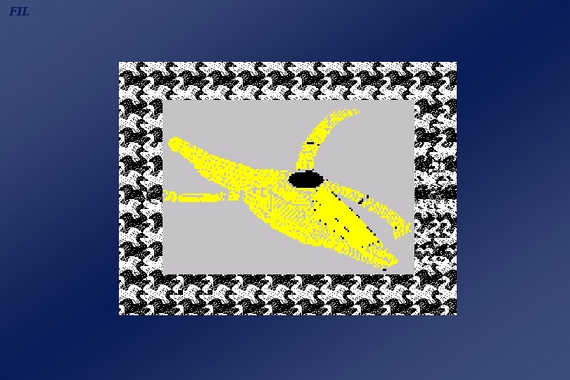
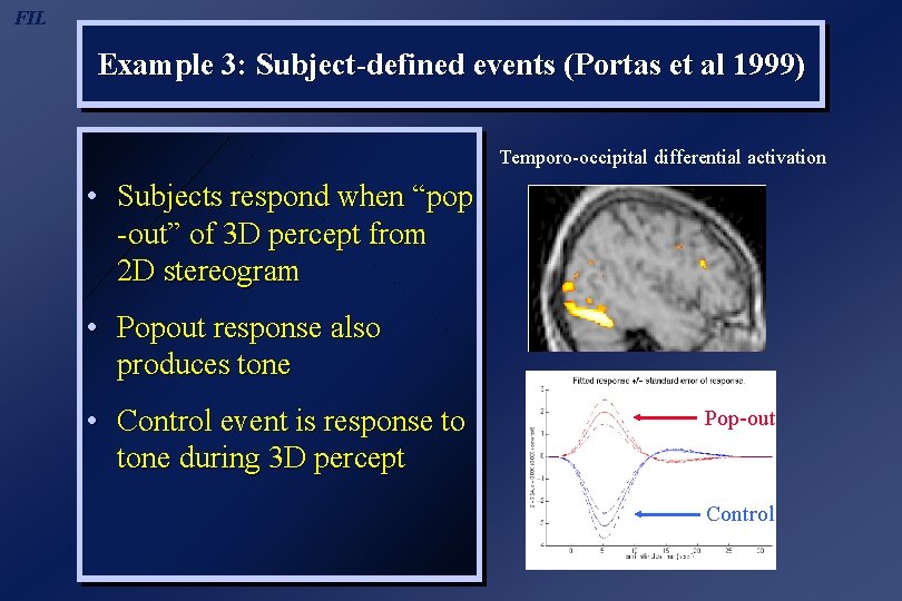
FIL Example 3: Subject-defined events (Portas et al 1999) • Subjects respond when “pop -out” of 3 D percept from 2 D stereogram

FIL

FIL Example 3: Subject-defined events (Portas et al 1999) Temporo-occipital differential activation • Subjects respond when “pop -out” of 3 D percept from 2 D stereogram • Popout response also produces tone • Control event is response to tone during 3 D percept Pop-out Control

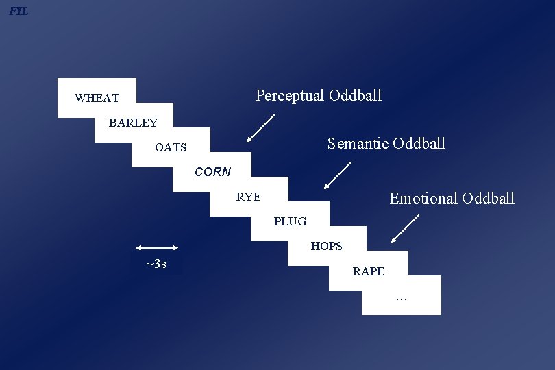
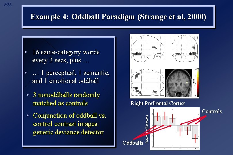
FIL Example 4: Oddball Paradigm (Strange et al, 2000) • 16 same-category words every 3 secs, plus … • … 1 perceptual, 1 semantic, and 1 emotional oddball

FIL Perceptual Oddball WHEAT BARLEY Semantic Oddball OATS CORN Emotional Oddball RYE PLUG HOPS ~3 s RAPE …

FIL Example 4: Oddball Paradigm (Strange et al, 2000) • 16 same-category words every 3 secs, plus … • … 1 perceptual, 1 semantic, and 1 emotional oddball Right Prefrontal Cortex Controls • Conjunction of oddball vs. control contrast images: generic deviance detector Oddballs Parameter Estimates • 3 nonoddballs randomly matched as controls

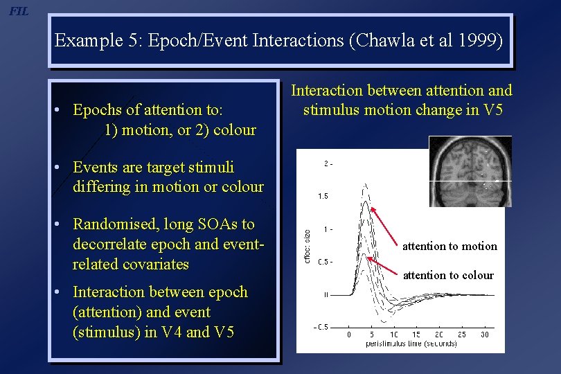
FIL Example 5: Epoch/Event Interactions (Chawla et al 1999) • Epochs of attention to: 1) motion, or 2) colour Interaction between attention and stimulus motion change in V 5 • Events are target stimuli differing in motion or colour • Randomised, long SOAs to decorrelate epoch and eventrelated covariates • Interaction between epoch (attention) and event (stimulus) in V 4 and V 5 attention to motion attention to colour

FIL