FIL SPM Course Oct 2012 VoxelBased Morphometry Ged

FIL SPM Course Oct 2012 Voxel-Based Morphometry Ged Ridgway, FIL/WTCN With thanks to John Ashburner
 • Spatial normalisation with Dartel")
Overview • Unified segmentation recap • Voxel-based morphometry (VBM) • Spatial normalisation with Dartel

Tissue segmentation • High-resolution MRI reveals fine structural detail in the • brain, but not all of it reliable or interesting • Noise, intensity-inhomogeneity, vasculature, … MR intensity is usually not quantitative (cf. relaxometry) • f. MRI time-series allow signal changes to be analysed statistically, compared to baseline or global values • Regional volumes of the three main tissue types: gray matter, white matter and CSF, are well-defined and potentially very interesting

Summary of unified segmentation • Unifies tissue segmentation and spatial normalisation • Principled Bayesian formulation: probabilistic generative model • Gaussian mixture model with deformable tissue prior probability maps (from segmentations in MNI space) • The inverse of the transformation that aligns the TPMs can be used to normalise the original image to standard space [Or the rigid component can be used to initialise Dartel] • • Intensity non-uniformity (bias) is included in the model
")
Tissue intensity distributions (T 1 -w MRI)
 • Classification is based on a Mixture")
Gaussian mixture model (GMM or Mo. G) • Classification is based on a Mixture of Gaussians (Mo. G) model fitted to the intensity probability density (histogram) Frequency Image Intensity

Modelling inhomogeneity • MR images are corrupted by spatially smooth • intensity variations (worse at high field strength) A multiplicative bias correction field is modelled as part of unified segmentation Corrupted image Bias Field Corrected image

TPMs – Tissue prior probability maps • Each TPM indicates the prior probability for a particular tissue at each point in MNI space • Fraction of occurrences in previous segmentations • TPMs are warped to match the subject • The inverse transform normalises to MNI space
 • Spatial normalisation with Dartel")
Overview • Unified segmentation • Voxel-based morphometry (VBM) • Spatial normalisation with Dartel

Computational neuroanatomy • Quantitative analysis of variability in biological shape • Can be univariate or multivariate, inferential or predictive • Example applications • • • Distinguish groups (e. g schizophrenics from healthy controls) Model changes (e. g. in development or aging) Characterise plasticity, e. g. when learning new skills Find structural correlates (scores, traits, genetics, etc. ) Differentiate degenerative disease from healthy aging • Evaluate subjects on drug treatments versus placebo

Voxel-Based Morphometry • Most widely used method for computational anatomy • VBM is essentially Statistical Parametric Mapping of regional segmented tissue density or volume • The exact interpretation of gray matter density or volume is complicated, and depends on the preprocessing steps used • It is not interpretable as neuronal packing density or other • cytoarchitectonic tissue properties The hope is that changes in these microscopic properties may lead to macro- or mesoscopic VBM-detectable differences

VBM methods overview • Unified segmentation and spatial normalisation • • • More flexible groupwise normalisation using DARTEL Volume-preserving transformation/warping Gaussian smoothing Optional computation of tissue totals/globals Voxel-wise statistical analysis

VBM in pictures Segment Normalise

VBM in pictures Segment Normalise Modulate Smooth

VBM in pictures Segment Normalise Modulate Smooth Voxel-wise statistics

VBM in pictures beta_0001 con_0001 Res. MS spm. T_0001 Segment Normalise Modulate Smooth Voxel-wise statistics FWE < 0. 05
 Native 1 intensity = tissue density 1 • Multiplication of the")
Modulation (“preserve amounts”) Native 1 intensity = tissue density 1 • Multiplication of the warped (normalised) tissue intensities so that their regional or global volume is preserved Unmodulated • Can detect differences in completely registered areas • Otherwise, we “preserve 1 1 concentrations”, and are detecting mesoscopic effects that remain after approximate registration has removed the macroscopic effects • Flexible (not necessarily “perfect”) Modulated registration may not leave any such differences 2/3 1/3 2/3
 • Top shows “unmodulated” data (wc 1), with intensity or concentration")
Modulation (“preserve amounts”) • Top shows “unmodulated” data (wc 1), with intensity or concentration preserved • Intensities are constant • Below is “modulated” data (mwc 1) with amounts or totals preserved • The voxel at the cross-hairs brightens as more tissue is compressed at this point

Smoothing • The analysis will be most sensitive to effects that match • • • the shape and size of the kernel The data will be more Gaussian and closer to a continuous random field for larger kernels • Usually recommend >= 6 mm Results will be rough and noise-like if too little smoothing is used Too much will lead to distributed, indistinct blobs • Usually recommend <= 12 mm
")
Smoothing as a locally weighted ROI • VBM > ROI: no subjective (or arbitrary) boundaries • VBM < ROI: harder to interpret blobs & characterise error

Interpreting findings Thinning Contrast Mis-register Thickening Folding Mis-classify

Interpreting findings VBM is sometimes described as “unbiased whole brain volumetry” Regional variation in registration accuracy Segmentation problems, issues with analysis mask Intensity, folding, etc. But significant blobs probably still indicate meaningful systematic effects!

Adjustment for “nuisance” variables • Anything which might explain some variability in regional volumes of interest should be considered • Age and gender are obvious and commonly used • Consider age+age 2 to allow quadratic effects • Site or scanner if more than one • (NB factor, not covariate!) Interval in longitudinal studies • Some “ 12 -month” intervals end up months longer… • Total grey matter volume often used for VBM • Changes interpretation when correlated with local • volumes (shape is a multivariate concept…) Total intracranial volume (TIV/ICV) sometimes more useful/interpretable, see also Barnes et al. , (2010), Neuro. Image 53(4): 1244 -55

Longitudinal VBM • The simplest method for longitudinal VBM is to use cross -sectional preprocessing, but longitudinal statistics • Standard preprocessing not optimal, but unbiased • Non-longitudinal statistics would inflate false positive rates • (Estimates of standard errors would be too small) • Simplest longitudinal statistical analysis: two-stage summary statistic approach (common in f. MRI) • Within subject longitudinal differences or beta estimates from linear regressions against time

Longitudinal VBM variations • Intra-subject registration over time is much more • • accurate than inter-subject normalisation A simple approach is to apply one set of normalisation parameters (e. g. estimated from baseline images) to both baseline and repeat(s) • Draganski et al (2004) Nature 427: 311 -312 More sophisticated approaches use nonlinear withinsubject registration, e. g. with HDW or new toolbox • E. g. Kipps et al (2005) JNNP 76: 650 • Beware of bias from asymmetries! (Thomas et al 2009) doi: 10. 1016/j. neuroimage. 2009. 05. 097
 • Spatial normalisation with Dartel")
Overview • Unified segmentation • Voxel-based morphometry (VBM) • Spatial normalisation with Dartel

Spatial normalisation with DARTEL • VBM is crucially dependent on registration performance • Limited flexibility (low Do. F) registration has been criticised • Inverse transformations are useful, but not always well-defined • More flexible registration requires careful modelling and regularisation (prior belief about reasonable warping) MNI/ICBM templates/priors are not universally representative • • The DARTEL toolbox combines several methodological advances to address these limitations • Evaluations show DARTEL performs at state-of-the art • E. g. Klein et al. , (2009) Neuro. Image 46(3): 786 -802 …

Part of Fig. 1 in Klein et al. Part of Fig. 5 in Klein et al.
 a flow u • Think syrup rather than")
DARTEL Transformations • Estimate (and regularise) a flow u • Think syrup rather than elastic • 3 (x, y, z) parameters per 1. 5 mm 3 voxel • 10^6 degrees of freedom vs. 10^3 DF for old discrete cosine basis functions • Scaling and squaring is used to • generate deformations Inverse simply integrates -u
 • Specific for matching tissue segments to")
DARTEL objective function • Likelihood component (matching) • Specific for matching tissue segments to their mean • Multinomial distribution (cf. Gaussian) • Prior component (regularisation) • A measure of deformation (flow) roughness = ½u. THu • Need to choose H and a balance between the two terms • Defaults usually work well (e. g. even for AD) • Though note that changing models (priors) can change results

Simultaneous registration of GM to GM and WM to WM, for a group of subjects Subject 1 Grey matter White matter Subject 2 Template Grey matter White matter Subject 4 Subject 3
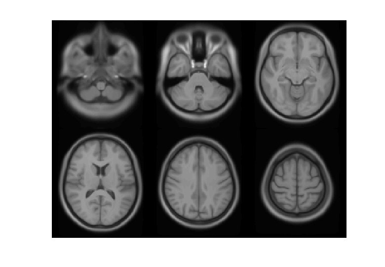
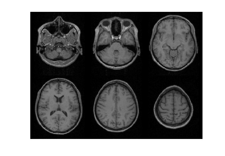
 Average of mwc 1 using")
DARTEL average template evolution Template 1 Rigid average (Template_0) Average of mwc 1 using segment/DCT Template 6
 normalised tissue segments")
Summary • VBM performs voxel-wise statistical analysis on • smoothed (modulated) normalised tissue segments SPM 8 performs segmentation and spatial normalisation in a unified generative model • Based on Gaussian mixture modelling, with DCT-warped • spatial priors, and multiplicative bias field The new segment toolbox includes non-brain priors and more flexible/precise warping of them • Subsequent (currently non-unified) use of DARTEL improves normalisation for VBM • And probably also f. MRI. . .

EXTRA MATERIAL

Mathematical advances in computational anatomy • VBM is well-suited to find focal volumetric differences • Assumes independence among voxels • Not very biologically plausible • But shows differences that are easy to interpret • Some anatomical differences can not be localised • Need multivariate models • Differences in terms of proportions among measurements • Where would the difference between male and female faces be localised?

Mathematical advances in computational anatomy • In theory, assumptions about structural covariance • among brain regions are more biologically plausible • Form influenced by spatio-temporal modes of gene expression Empirical evidence, e. g. • Mechelli, Friston, Frackowiak & Price. Structural covariance in the human cortex. Journal of Neuroscience 25: 8303 -10 (2005) • Recent introductory review: • Ashburner & Klöppel. “Multivariate models of inter-subject anatomical variability”. Neuro. Image 56(2): 422 -439 (2011)

Summary of extra material • VBM uses the machinery of SPM to localise patterns in regional volumetric variation • Use of “globals” as covariates is a step towards multivariate modelling of volume and shape • More advanced approaches typically benefit from the • • same preprocessing methods • New segmentation and DARTEL close to state of the art • Though possibly little or no smoothing Elegant mathematics related to transformations (diffeomorphism group with Riemannian metric) VBM – easier interpretation – complementary role

Historical bibliography of VBM • A Voxel-Based Method for the Statistical Analysis of Gray and White Matter Density… Wright, Mc. Guire, Poline, Travere, Murrary, Frith, Frackowiak and Friston (1995 (!)) Neuro. Image 2(4) • Rigid reorientation (by eye), semi-automatic scalp editing and segmentation, 8 mm smoothing, SPM statistics, global covars. • Voxel-Based Morphometry – The Methods. Ashburner and Friston (2000) Neuro. Image 11(6 pt. 1) • Non-linear spatial normalisation, automatic segmentation • Thorough consideration of assumptions and confounds

Historical bibliography of VBM • A Voxel-Based Morphometric Study of Ageing… Good, • Johnsrude, Ashburner, Henson and Friston (2001) Neuro. Image 14(1) • Optimised GM-normalisation (“a half-baked procedure”) Unified Segmentation. Ashburner and Friston (2005) Neuro. Image 26(3) • Principled generative model for segmentation using deformable priors • A Fast Diffeomorphic Image Registration Algorithm. • Ashburner (2007) Neuroimage 38(1) • Large deformation normalisation Computing average shaped tissue probability templates. Ashburner & Friston (2009) Neuro. Image 45(2): 333 -341
- Slides: 41