Eventrelated f MRI Guillaume Flandin Wellcome Trust Centre

Event-related f. MRI Guillaume Flandin Wellcome Trust Centre for Neuroimaging University College London SPM Course Chicago, 22 -23 Oct 2015

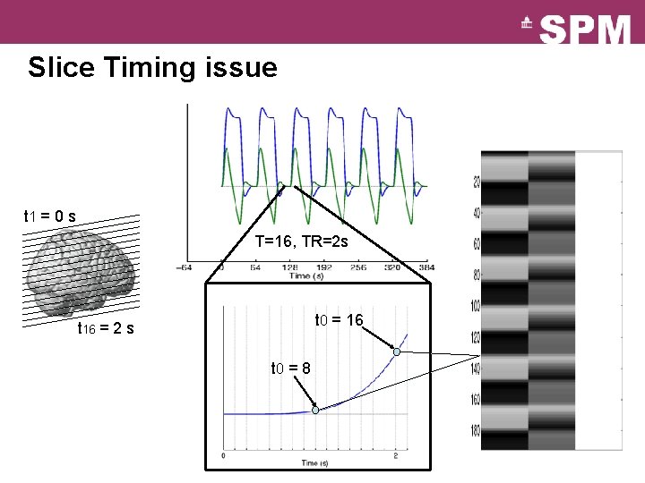
Slice Timing issue t 1 = 0 s T=16, TR=2 s t 0 = 16 t 16 = 2 s t 0 = 8

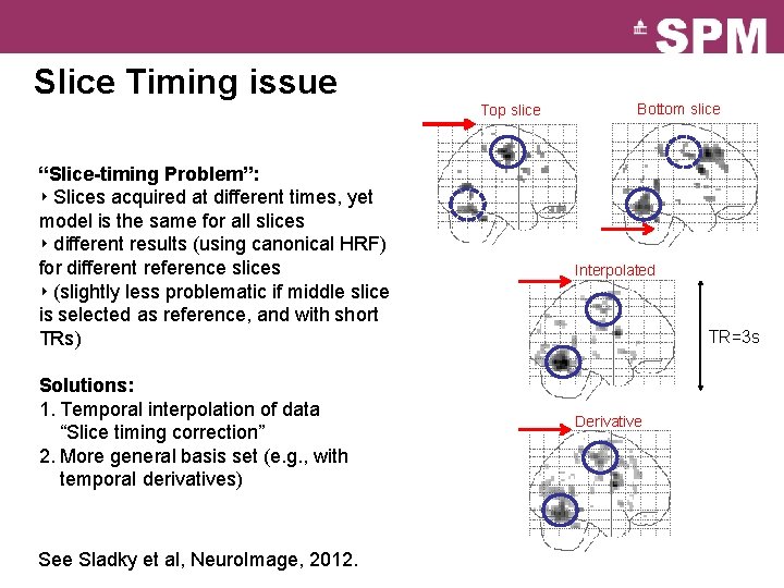
Slice Timing issue Top slice “Slice-timing Problem”: ‣ Slices acquired at different times, yet model is the same for all slices ‣ different results (using canonical HRF) for different reference slices ‣ (slightly less problematic if middle slice is selected as reference, and with short TRs) Solutions: 1. Temporal interpolation of data “Slice timing correction” 2. More general basis set (e. g. , with temporal derivatives) See Sladky et al, Neuro. Image, 2012. Bottom slice Interpolated TR=3 s Derivative

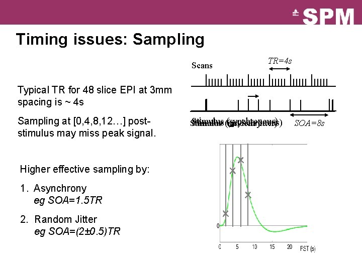
Timing issues: Sampling Scans TR=4 s Typical TR for 48 slice EPI at 3 mm spacing is ~ 4 s Sampling at [0, 4, 8, 12…] post- stimulus may miss peak signal. Higher effective sampling by: 1. Asynchrony eg SOA=1. 5 TR 2. Random Jitter eg SOA=(2± 0. 5)TR Stimulus (random (synchronous) (asynchronous) Stimulus jitter) SOA=8 s

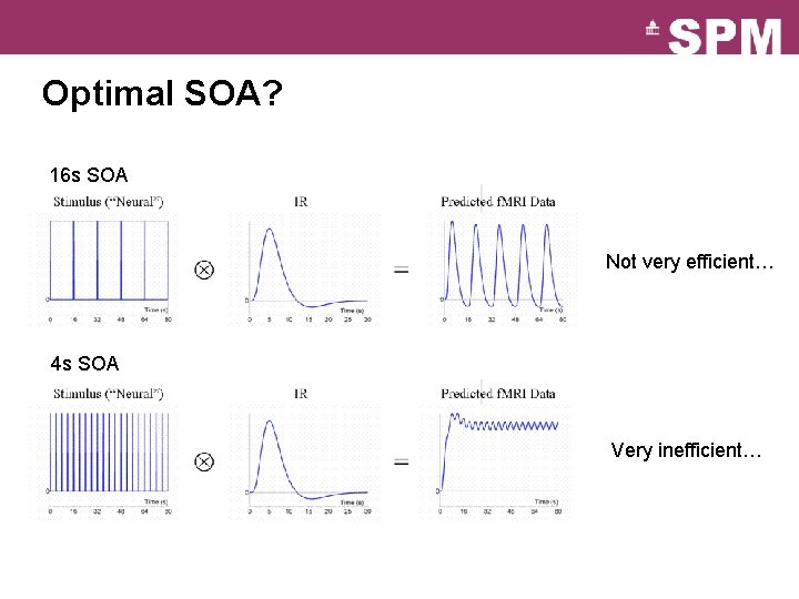
Optimal SOA? 16 s SOA Not very efficient… 4 s SOA Very inefficient…

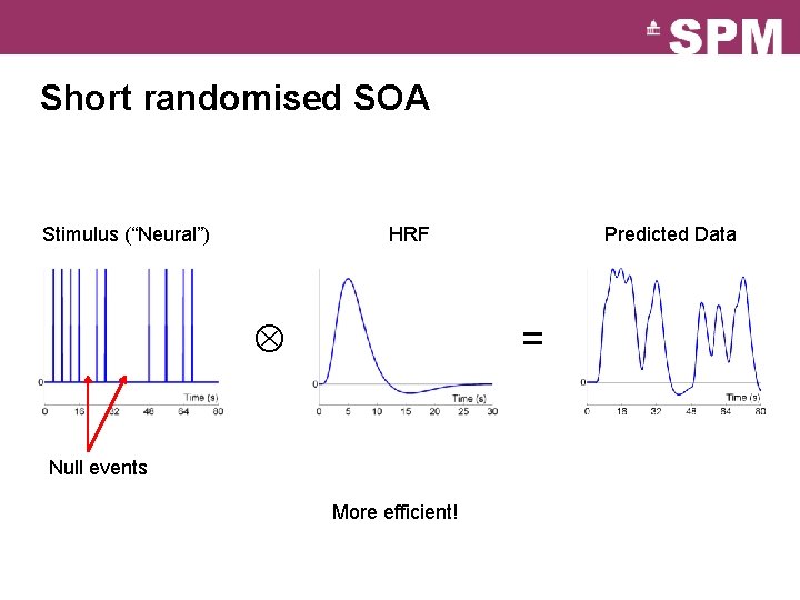
Short randomised SOA Stimulus (“Neural”) HRF Predicted Data = Null events More efficient!

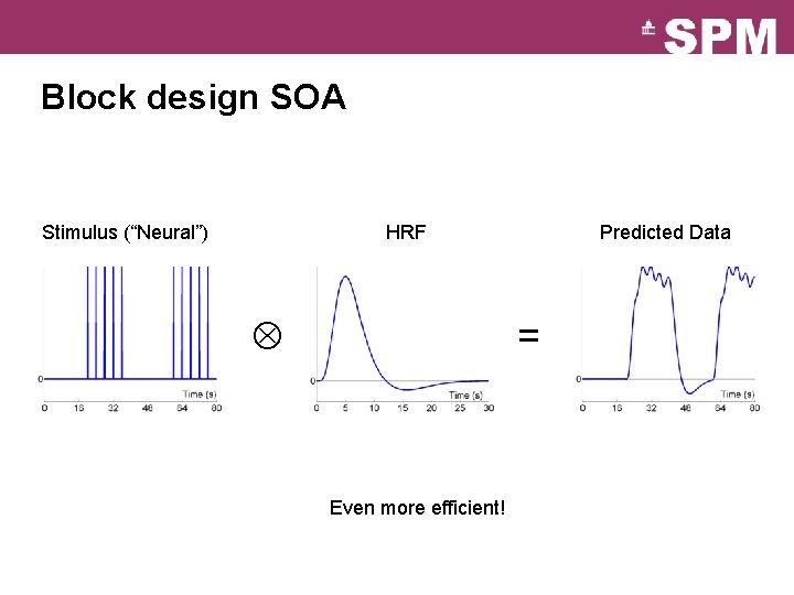
Block design SOA Stimulus (“Neural”) HRF Predicted Data = Even more efficient!

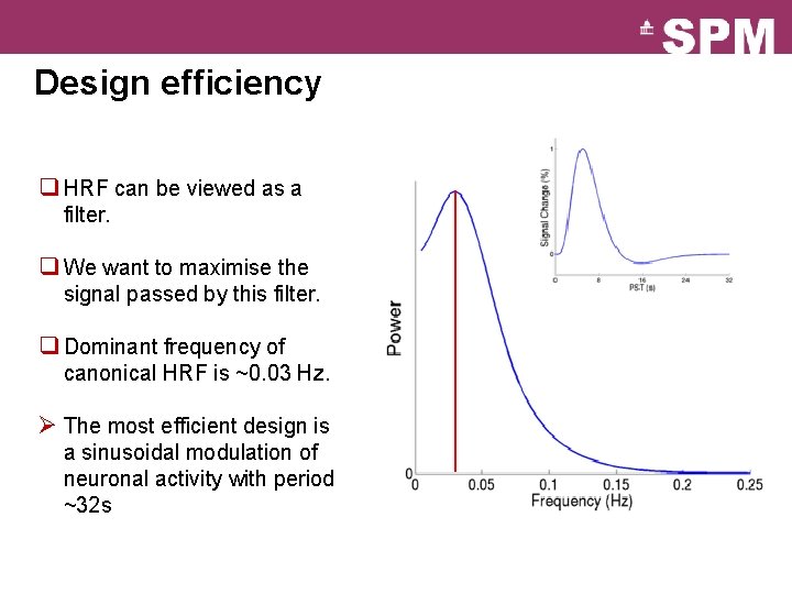
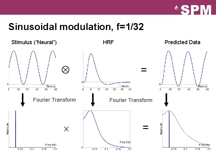
Design efficiency q HRF can be viewed as a filter. q We want to maximise the signal passed by this filter. q Dominant frequency of canonical HRF is ~0. 03 Hz. Ø The most efficient design is a sinusoidal modulation of neuronal activity with period ~32 s

Sinusoidal modulation, f=1/32 Stimulus (“Neural”) HRF Fourier Transform Predicted Data = = Fourier Transform =

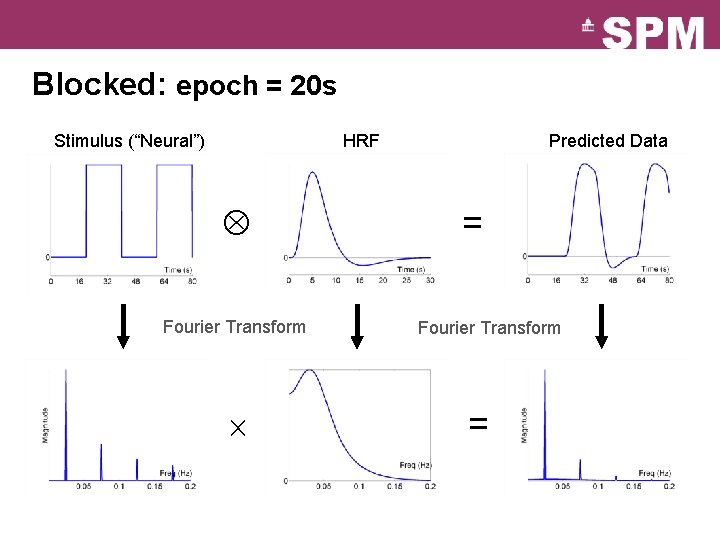
Blocked: epoch = 20 s Stimulus (“Neural”) HRF Fourier Transform Predicted Data = Fourier Transform =

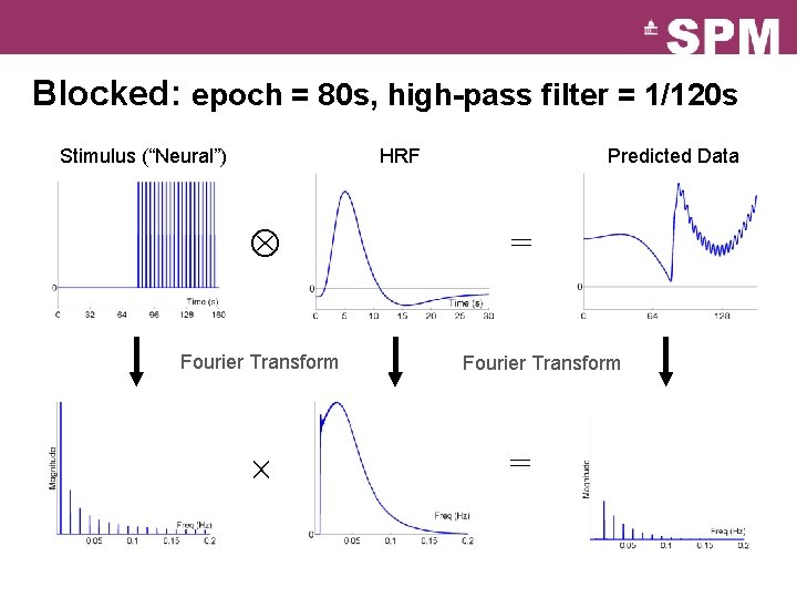
Blocked: epoch = 80 s, high-pass filter = 1/120 s Stimulus (“Neural”) HRF Fourier Transform Predicted Data = Fourier Transform =

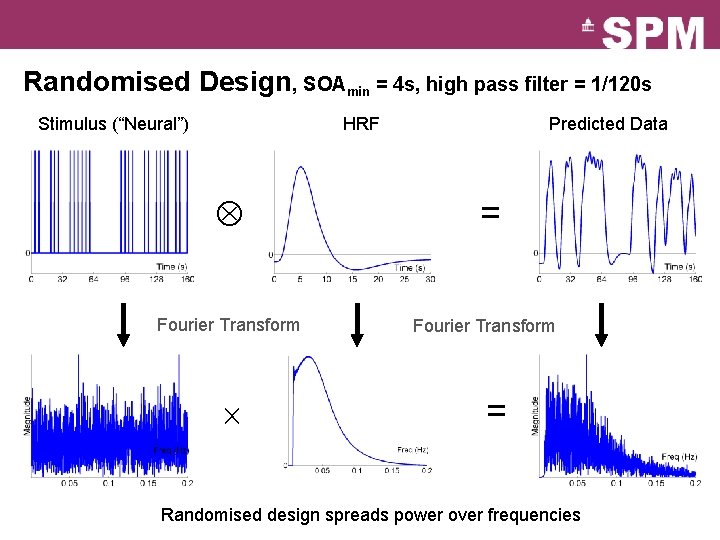
Randomised Design, SOAmin = 4 s, high pass filter = 1/120 s Stimulus (“Neural”) HRF Fourier Transform Predicted Data = Fourier Transform = Randomised design spreads power over frequencies

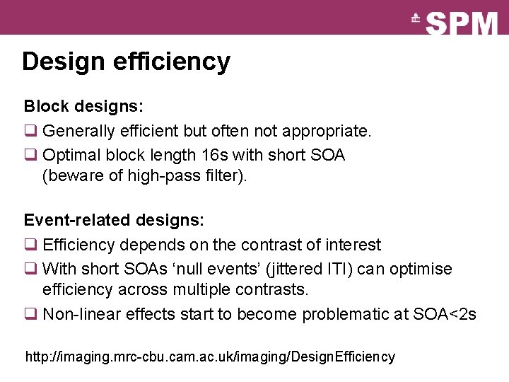
Design efficiency Block designs: q Generally efficient but often not appropriate. q Optimal block length 16 s with short SOA (beware of high-pass filter). Event-related designs: q Efficiency depends on the contrast of interest q With short SOAs ‘null events’ (jittered ITI) can optimise efficiency across multiple contrasts. q Non-linear effects start to become problematic at SOA<2 s http: //imaging. mrc-cbu. cam. ac. uk/imaging/Design. Efficiency

Multiple testing (random field theory) Guillaume Flandin Wellcome Trust Centre for Neuroimaging University College London SPM Course Chicago, 22 -23 Oct 2015

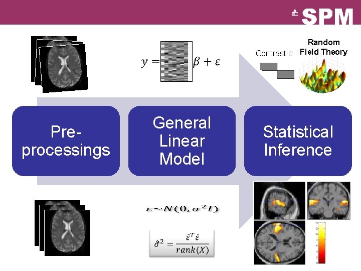
Random Contrast c Field Theory General Linear Model Preprocessings Statistical Inference

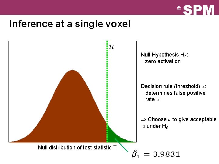
Inference at a single voxel u Null Hypothesis H 0: zero activation Decision rule (threshold) u: determines false positive rate α Choose u to give acceptable α under H 0 Null distribution of test statistic T

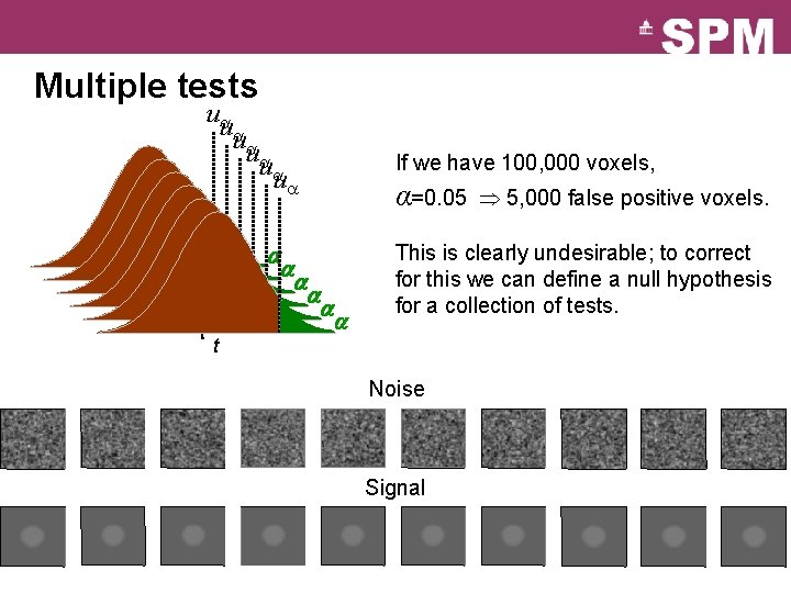
Multiple tests u u u t t t If we have 100, 000 voxels, α=0. 05 5, 000 false positive voxels. This is clearly undesirable; to correct for this we can define a null hypothesis for a collection of tests. t Noise Signal

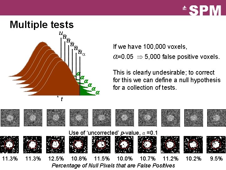
Multiple tests u u u t t t If we have 100, 000 voxels, α=0. 05 5, 000 false positive voxels. This is clearly undesirable; to correct for this we can define a null hypothesis for a collection of tests. t Use of ‘uncorrected’ p-value, α =0. 1 11. 3% 12. 5% 10. 8% 11. 5% 10. 0% 10. 7% 11. 2% Percentage of Null Pixels that are False Positives 10. 2% 9. 5%

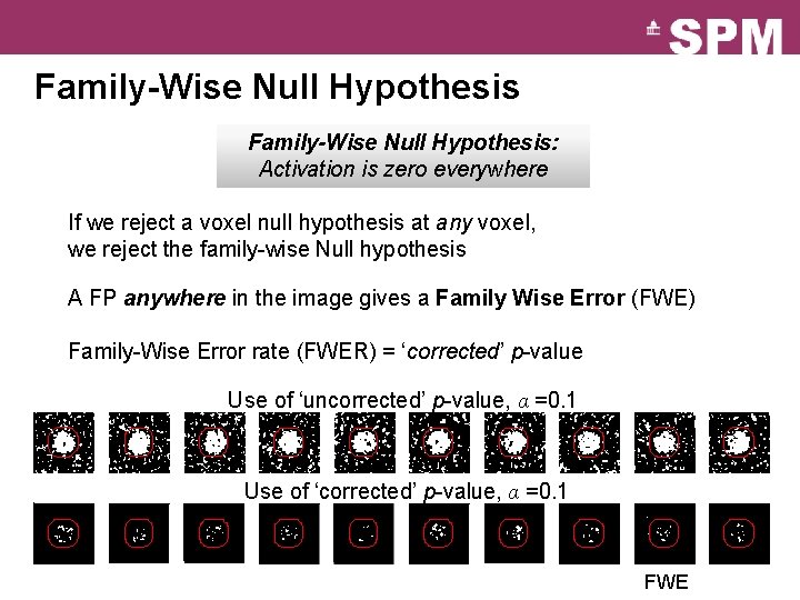
Family-Wise Null Hypothesis: Activation is zero everywhere If we reject a voxel null hypothesis at any voxel, we reject the family-wise Null hypothesis A FP anywhere in the image gives a Family Wise Error (FWE) Family-Wise Error rate (FWER) = ‘corrected’ p-value Use of ‘uncorrected’ p-value, α =0. 1 Use of ‘corrected’ p-value, α =0. 1 FWE

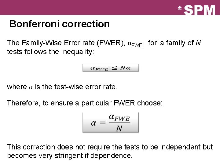
Bonferroni correction The Family-Wise Error rate (FWER), αFWE, for a family of N tests follows the inequality: where α is the test-wise error rate. Therefore, to ensure a particular FWER choose: This correction does not require the tests to be independent but becomes very stringent if dependence.

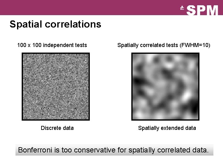
Spatial correlations 100 x 100 independent tests Discrete data Spatially correlated tests (FWHM=10) Spatially extended data Bonferroni is too conservative for spatially correlated data.

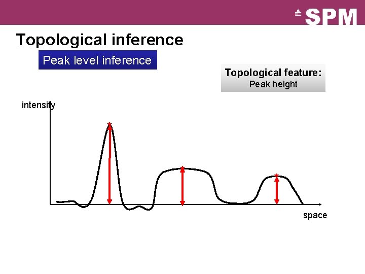
Topological inference Peak level inference Topological feature: Peak height intensity space

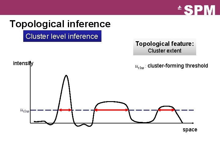
Topological inference Cluster level inference Topological feature: Cluster extent intensity uclus : cluster-forming threshold uclus space

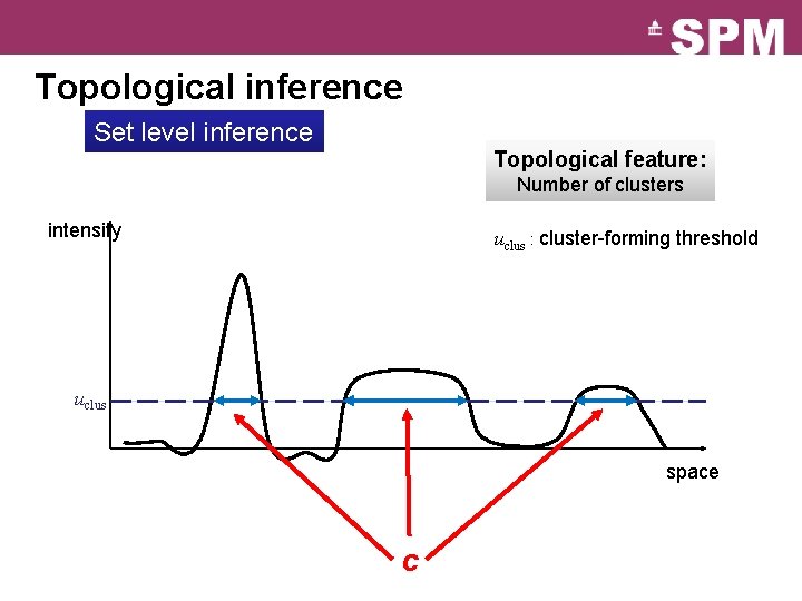
Topological inference Set level inference Topological feature: Number of clusters intensity uclus : cluster-forming threshold uclus space c

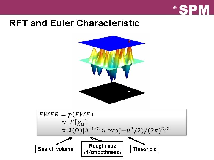
RFT and Euler Characteristic Search volume Roughness (1/smoothness) Threshold

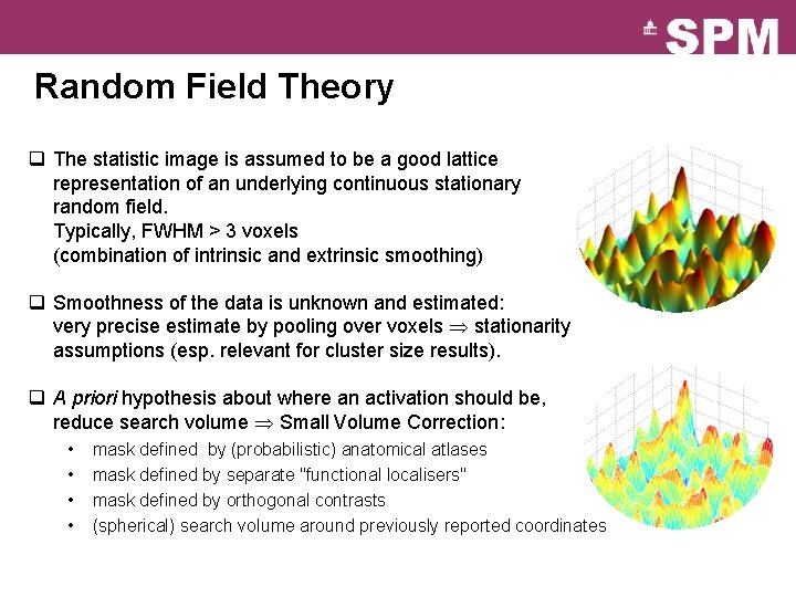
Random Field Theory q The statistic image is assumed to be a good lattice representation of an underlying continuous stationary random field. Typically, FWHM > 3 voxels (combination of intrinsic and extrinsic smoothing) q Smoothness of the data is unknown and estimated: very precise estimate by pooling over voxels stationarity assumptions (esp. relevant for cluster size results). q A priori hypothesis about where an activation should be, reduce search volume Small Volume Correction: • • mask defined by (probabilistic) anatomical atlases mask defined by separate "functional localisers" mask defined by orthogonal contrasts (spherical) search volume around previously reported coordinates

Conclusion q There is a multiple testing problem and corrections have to be applied on p-values (for the volume of interest only (see Small Volume Correction)). q Inference is made about topological features (peak height, spatial extent, number of clusters). Use results from the Random Field Theory. q Control of FWER (probability of a false positive anywhere in the image): very specific, not so sensitive. q Control of FDR (expected proportion of false positives amongst those features declared positive (the discoveries)): less specific, more sensitive.

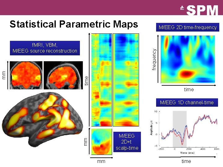
Statistical Parametric Maps frequency time mm f. MRI, VBM, M/EEG source reconstruction M/EEG 2 D time-frequency time mm M/EEG 1 D channel-time M/EEG 2 D+t scalp-time mm mm mm time

Group Analyses Guillaume Flandin Wellcome Trust Centre for Neuroimaging University College London SPM Course Chicago, 22 -23 Oct 2015

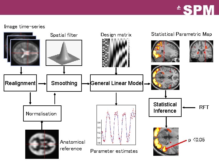
Image time-series Realignment Spatial filter Design matrix Smoothing General Linear Model Statistical Parametric Map Statistical Inference Normalisation Anatomical reference Parameter estimates RFT p <0. 05

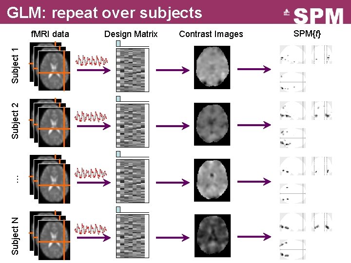
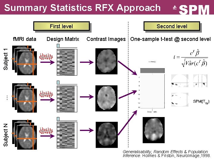
GLM: repeat over subjects Subject N … Subject 2 Subject 1 f. MRI data Design Matrix Contrast Images SPM{t}

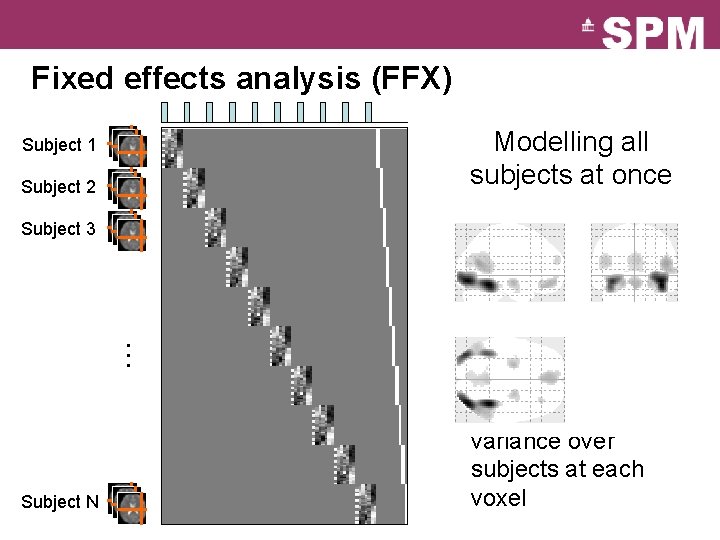
Fixed effects analysis (FFX) Modelling all subjects at once Subject 1 Subject 2 þ Simple model þ Lots of degrees of Subject 3 … freedom Subject N ý Large amount of data ý Assumes common variance over subjects at each voxel

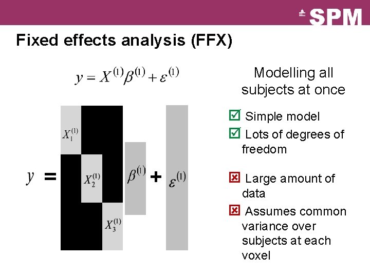
Fixed effects analysis (FFX) Modelling all subjects at once þ Simple model þ Lots of degrees of freedom = + ý Large amount of data ý Assumes common variance over subjects at each voxel

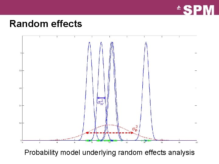
Random effects Probability model underlying random effects analysis

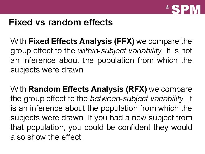
Fixed vs random effects With Fixed Effects Analysis (FFX) we compare the group effect to the within-subject variability. It is not an inference about the population from which the subjects were drawn. With Random Effects Analysis (RFX) we compare the group effect to the between-subject variability. It is an inference about the population from which the subjects were drawn. If you had a new subject from that population, you could be confident they would also show the effect.

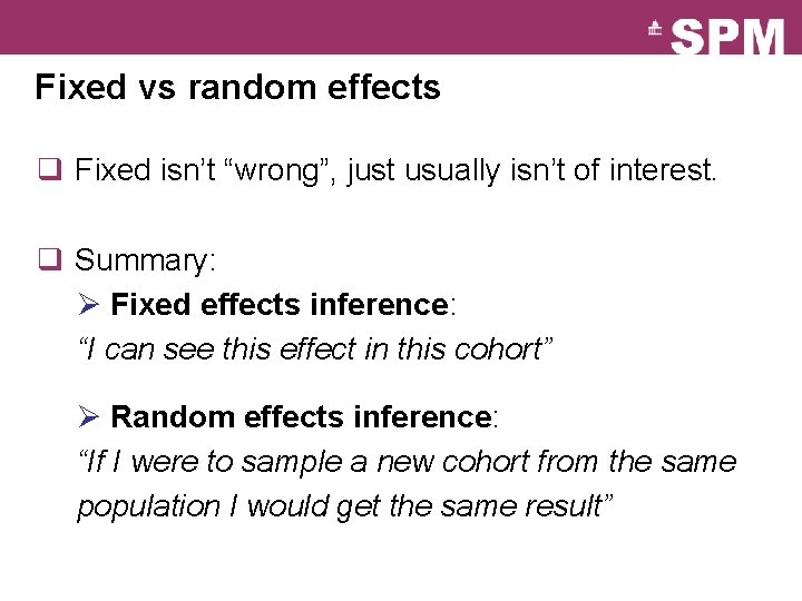
Fixed vs random effects q Fixed isn’t “wrong”, just usually isn’t of interest. q Summary: Ø Fixed effects inference: “I can see this effect in this cohort” Ø Random effects inference: “If I were to sample a new cohort from the same population I would get the same result”

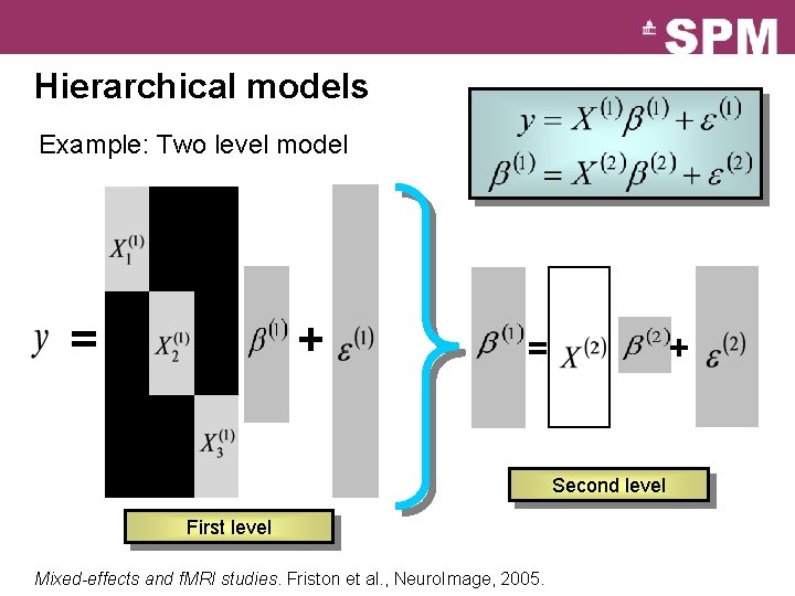
Hierarchical models Example: Two level model = + + = Second level First level Mixed-effects and f. MRI studies. Friston et al. , Neuro. Image, 2005.

Summary Statistics RFX Approach First level Design Matrix Contrast Images One-sample t-test @ second level Subject N … Subject 1 f. MRI data Second level Generalisability, Random Effects & Population Inference. Holmes & Friston, Neuro. Image, 1998.

Summary Statistics RFX Approach Assumptions q The summary statistics approach is exact if for each session/subject: Ø Within-subjects variances the same Ø First level design the same (e. g. number of trials) q Other cases: summary statistics approach is robust against typical violations. Mixed-effects and f. MRI studies. Friston et al. , Neuro. Image, 2005. Statistical Parametric Mapping: The Analysis of Functional Brain Images. Elsevier, 2007. Simple group f. MRI modeling and inference. Mumford & Nichols. Neuro. Image, 2009.

ANOVA & non-sphericity q One effect per subject: Ø Summary statistics approach Ø One-sample t-test at the second level q More than one effect per subject or multiple groups: Ø Non-sphericity modelling Ø Covariance components and Re. ML

Summary q Group Inference usually proceeds with RFX analysis, not FFX. Group effects are compared to between rather than within subject variability. q Hierarchical models provide a gold-standard for RFX analysis but are computationally intensive. q Summary statistics approach is a robust method for RFX group analysis. q Can also use ‘ANOVA’ or ‘ANOVA within subject’ at second level for inference about multiple experimental conditions or multiple groups.

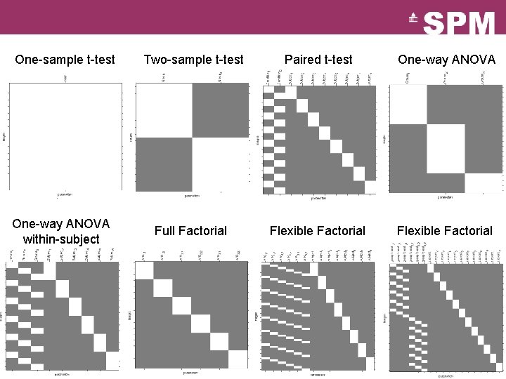
One-sample t-test Two-sample t-test Paired t-test One-way ANOVA within-subject Full Factorial Flexible Factorial

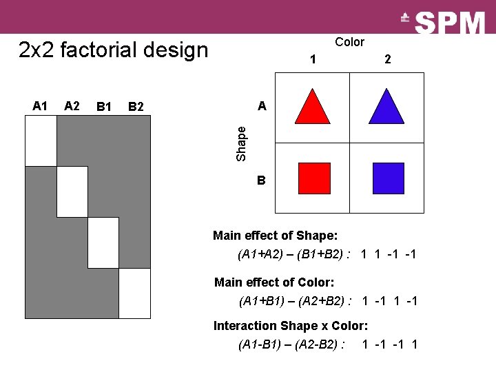
Color 2 x 2 factorial design A 2 B 1 2 A B 2 Shape A 1 1 B Main effect of Shape: (A 1+A 2) – (B 1+B 2) : 1 1 -1 -1 Main effect of Color: (A 1+B 1) – (A 2+B 2) : 1 -1 Interaction Shape x Color: (A 1 -B 1) – (A 2 -B 2) : 1 -1 -1 1

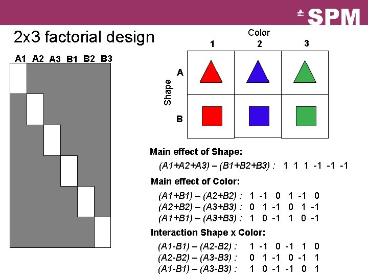
2 x 3 factorial design 1 Color 2 3 A 1 A 2 A 3 B 1 B 2 B 3 Shape A B Main effect of Shape: (A 1+A 2+A 3) – (B 1+B 2+B 3) : 1 1 1 -1 -1 -1 Main effect of Color: (A 1+B 1) – (A 2+B 2) : 1 -1 0 (A 2+B 2) – (A 3+B 3) : 0 1 -1 (A 1+B 1) – (A 3+B 3) : 1 0 -1 Interaction Shape x Color: (A 1 -B 1) – (A 2 -B 2) : 1 -1 0 -1 1 0 (A 2 -B 2) – (A 3 -B 3) : 0 1 -1 0 -1 1 (A 1 -B 1) – (A 3 -B 3) : 1 0 -1 -1 0 1