Topological Inference Guillaume Flandin Wellcome Centre for Human

Topological Inference Guillaume Flandin Wellcome Centre for Human Neuroimaging University College London SPM Course London, May 2019

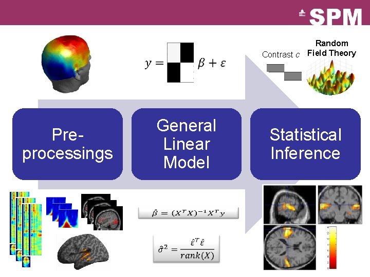
Random Contrast c Field Theory General Linear Model Preprocessings Statistical Inference

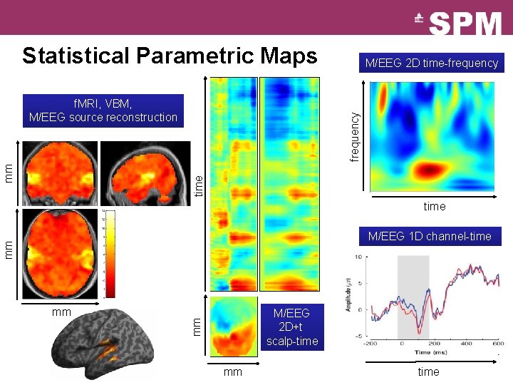
Statistical Parametric Maps frequency time mm f. MRI, VBM, M/EEG source reconstruction M/EEG 2 D time-frequency time mm M/EEG 1 D channel-time M/EEG 2 D+t scalp-time mm mm mm time

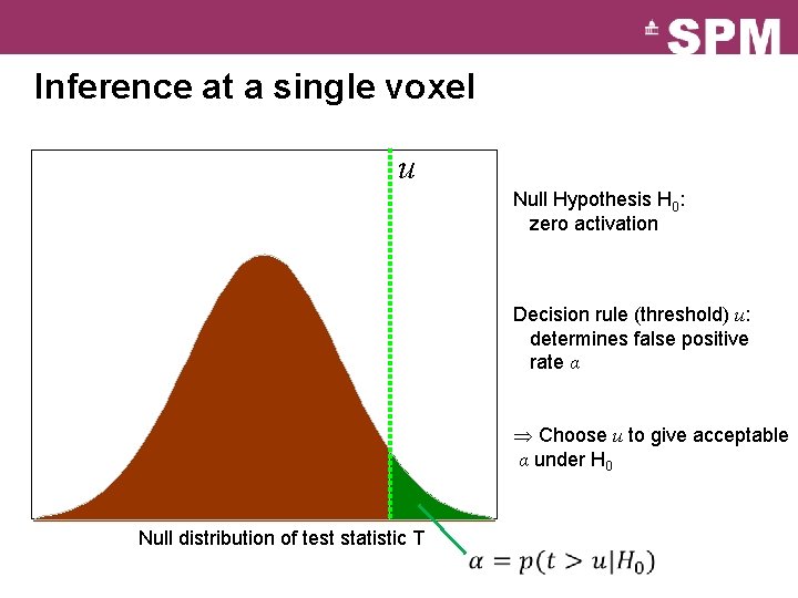
Inference at a single voxel u Null Hypothesis H 0: zero activation Decision rule (threshold) u: determines false positive rate α Choose u to give acceptable α under H 0 Null distribution of test statistic T

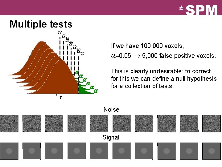
Multiple tests u u u t t t If we have 100, 000 voxels, α=0. 05 5, 000 false positive voxels. This is clearly undesirable; to correct for this we can define a null hypothesis for a collection of tests. t Noise Signal

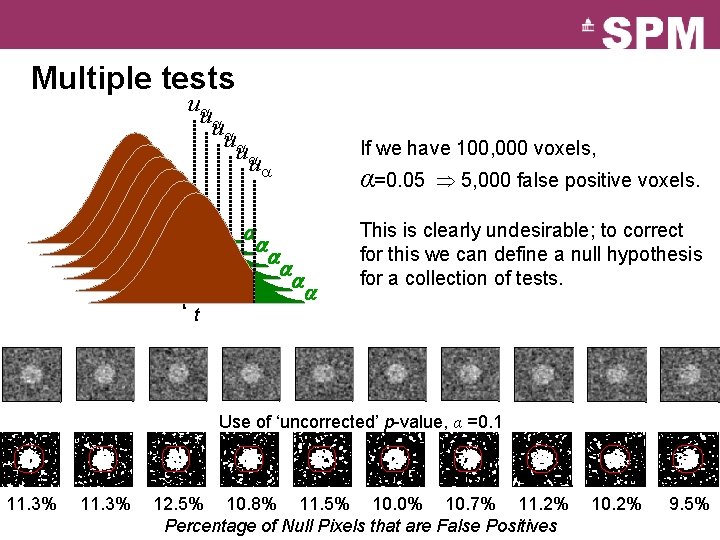
Multiple tests u u u t t t If we have 100, 000 voxels, α=0. 05 5, 000 false positive voxels. This is clearly undesirable; to correct for this we can define a null hypothesis for a collection of tests. t Use of ‘uncorrected’ p-value, α =0. 1 11. 3% 12. 5% 10. 8% 11. 5% 10. 0% 10. 7% 11. 2% Percentage of Null Pixels that are False Positives 10. 2% 9. 5%

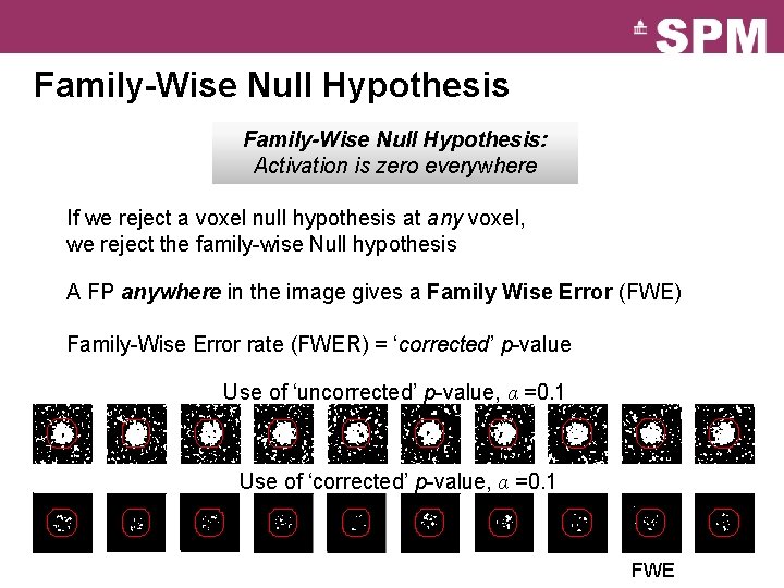
Family-Wise Null Hypothesis: Activation is zero everywhere If we reject a voxel null hypothesis at any voxel, we reject the family-wise Null hypothesis A FP anywhere in the image gives a Family Wise Error (FWE) Family-Wise Error rate (FWER) = ‘corrected’ p-value Use of ‘uncorrected’ p-value, α =0. 1 Use of ‘corrected’ p-value, α =0. 1 FWE

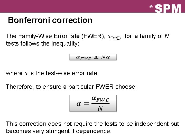
Bonferroni correction The Family-Wise Error rate (FWER), αFWE, for a family of N tests follows the inequality: where α is the test-wise error rate. Therefore, to ensure a particular FWER choose: This correction does not require the tests to be independent but becomes very stringent if dependence.

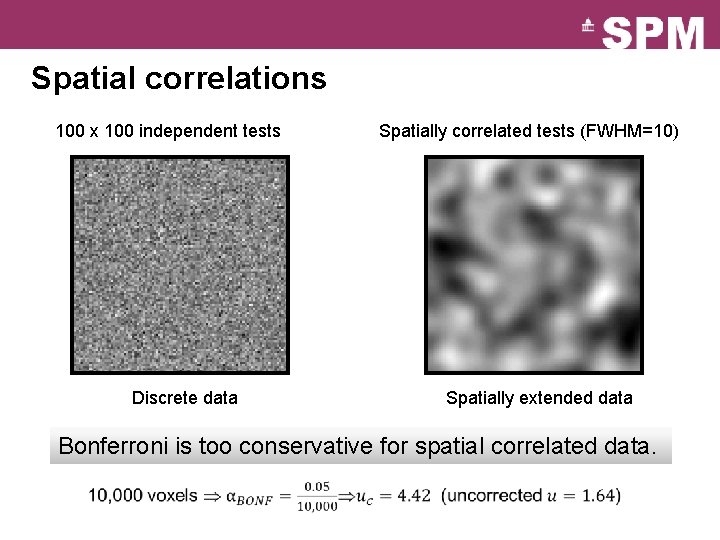
Spatial correlations 100 x 100 independent tests Discrete data Spatially correlated tests (FWHM=10) Spatially extended data Bonferroni is too conservative for spatial correlated data.

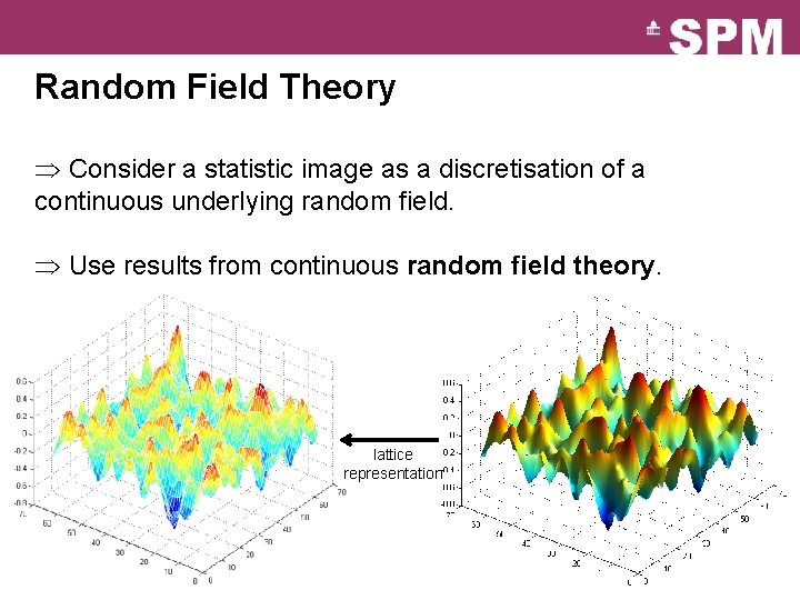
Random Field Theory Consider a statistic image as a discretisation of a continuous underlying random field. Use results from continuous random field theory. lattice representation

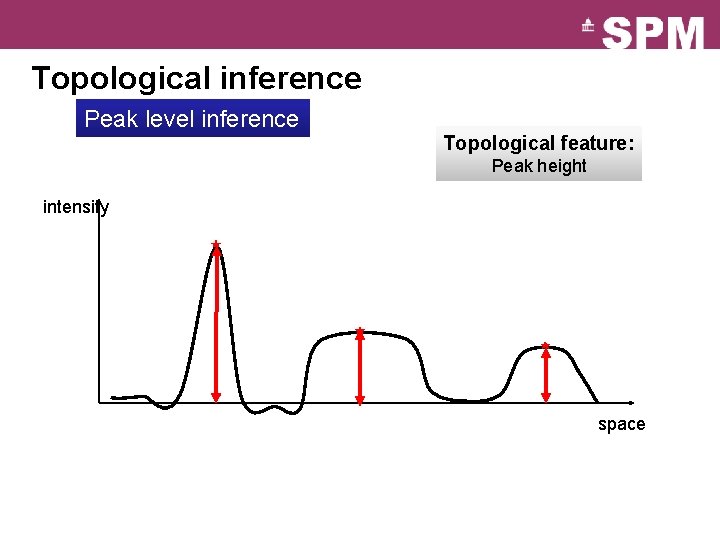
Topological inference Peak level inference Topological feature: Peak height intensity space

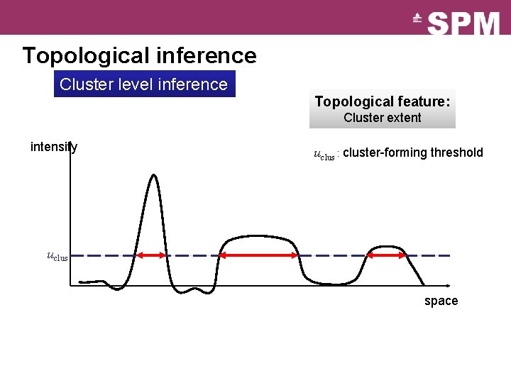
Topological inference Cluster level inference Topological feature: Cluster extent intensity uclus : cluster-forming threshold uclus space

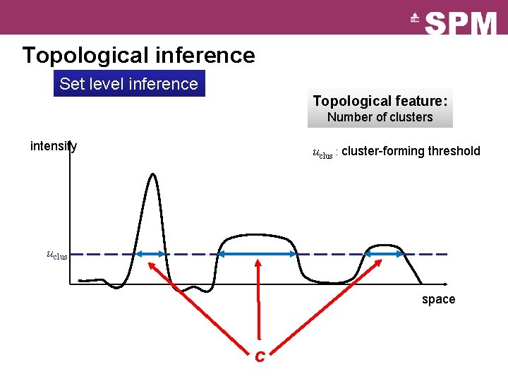
Topological inference Set level inference Topological feature: Number of clusters intensity uclus : cluster-forming threshold uclus space c

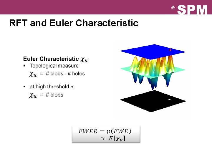
RFT and Euler Characteristic

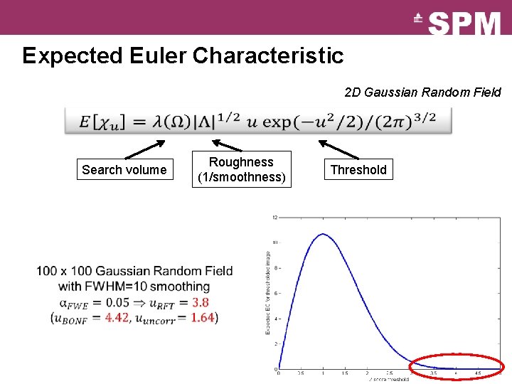
Expected Euler Characteristic 2 D Gaussian Random Field Search volume Roughness (1/smoothness) Threshold

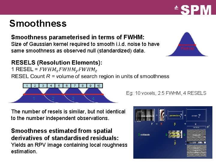
Smoothness parameterised in terms of FWHM: Size of Gaussian kernel required to smooth i. i. d. noise to have same smoothness as observed null (standardized) data. FWHM 1 2 3 4 5 6 7 8 9 10 Eg: 10 voxels, 2. 5 FWHM, 4 RESELS 1 2 3 4 The number of resels is similar, but not identical to the number independent observations. Smoothness estimated from spatial derivatives of standardised residuals: Yields an RPV image containing local roughness estimation.

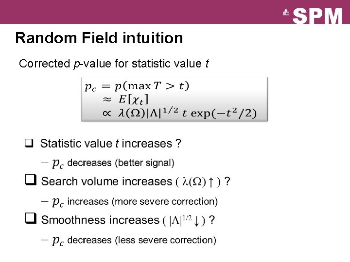
Random Field intuition Corrected p-value for statistic value t

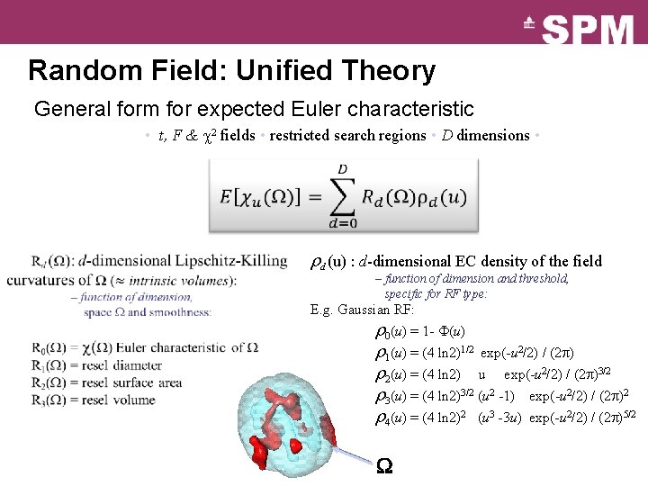
Random Field: Unified Theory General form for expected Euler characteristic • t, F & 2 fields • restricted search regions • D dimensions • rd (u) : d-dimensional EC density of the field – function of dimension and threshold, specific for RF type: E. g. Gaussian RF: r 0(u) = 1 - (u) r 1(u) = (4 ln 2)1/2 exp(-u 2/2) / (2 p) r 2(u) = (4 ln 2) u exp(-u 2/2) / (2 p)3/2 r 3(u) = (4 ln 2)3/2 (u 2 -1) exp(-u 2/2) / (2 p)2 r 4(u) = (4 ln 2)2 (u 3 -3 u) exp(-u 2/2) / (2 p)5/2

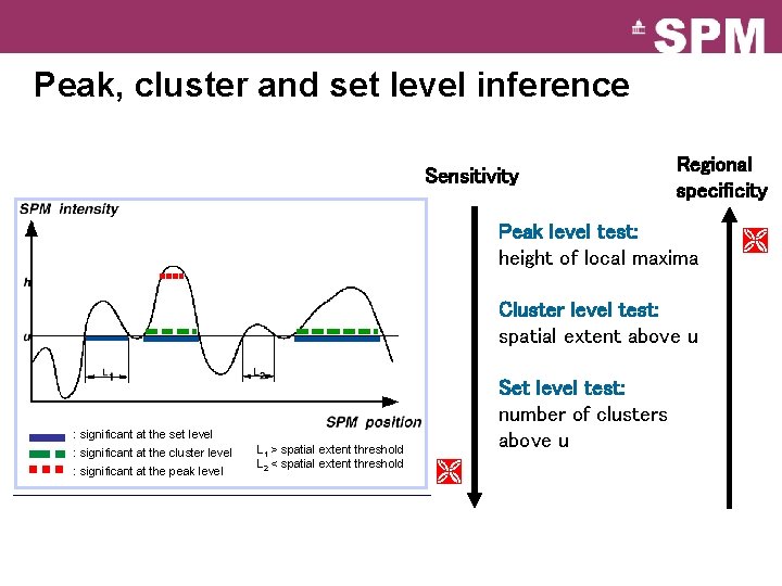
Peak, cluster and set level inference Sensitivity Regional specificity Peak level test: height of local maxima Cluster level test: spatial extent above u Set level test: number of clusters above u : significant at the set level : significant at the cluster level : significant at the peak level L 1 > spatial extent threshold L 2 < spatial extent threshold

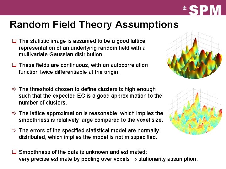
Random Field Theory Assumptions q The statistic image is assumed to be a good lattice representation of an underlying random field with a multivariate Gaussian distribution. q These fields are continuous, with an autocorrelation function twice differentiable at the origin. ð The threshold chosen to define clusters is high enough such that the expected EC is a good approximation to the number of clusters. ð The lattice approximation is reasonable, which implies the smoothness is relatively large compared to the voxel size. ð The errors of the specified statistical model are normally distributed, which implies the model is not misspecified. q Smoothness of the data is unknown and estimated: very precise estimate by pooling over voxels stationarity assumption.

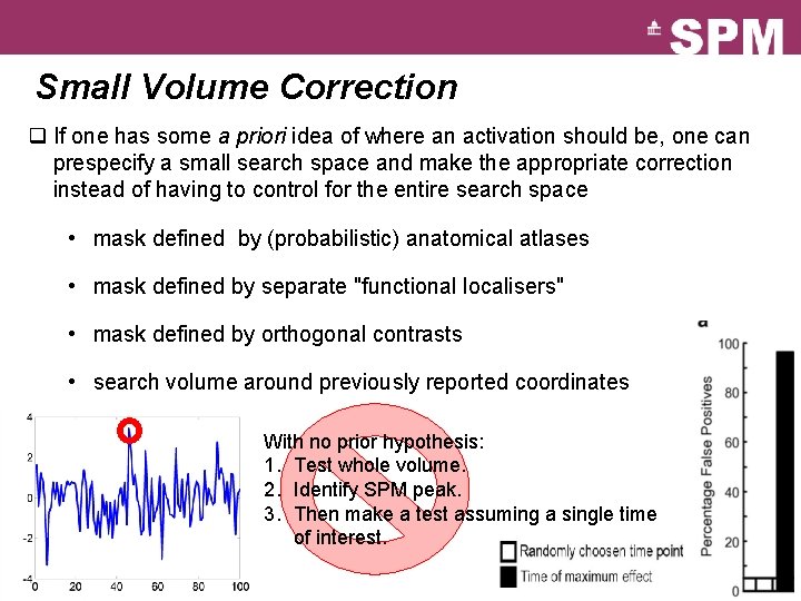
Small Volume Correction q If one has some a priori idea of where an activation should be, one can prespecify a small search space and make the appropriate correction instead of having to control for the entire search space • mask defined by (probabilistic) anatomical atlases • mask defined by separate "functional localisers" • mask defined by orthogonal contrasts • search volume around previously reported coordinates With no prior hypothesis: 1. Test whole volume. 2. Identify SPM peak. 3. Then make a test assuming a single time of interest.

Conclusion q There is a multiple testing problem and corrections have to be applied on p-values (for the volume of interest only (see SVC)). q Inference is made about topological features (peak height, spatial extent, number of clusters). Use results from the Random Field Theory. q Control of FWER (probability of a false positive anywhere in the image) for a space of any dimension and shape. Many thanks to Justin Chumbley, Tom Nichols and Gareth Barnes for slides

References q Friston KJ, Frith CD, Liddle PF, Frackowiak RS. Comparing functional (PET) images: the assessment of significant change. Journal of Cerebral Blood Flow and Metabolism, 1991. q Worsley KJ, Evans AC, Marrett S, Neelin P. A three-dimensional statistical analysis for CBF activation studies in human brain. Journal of Cerebral Blood Flow and Metabolism. 1992. q Worsley KJ, Marrett S, Neelin P, Vandal AC, Friston KJ, Evans AC. A unified statistical approach for determining significant signals in images of cerebral activation. Human Brain Mapping, 1996. q Chumbley J, Worsley KJ , Flandin G, and Friston KJ. Topological FDR for neuroimaging. Neuro. Image, 2010. q Kilner J and Friston KJ. Topological inference for EEG and MEG data. Annals of Applied Statistics, 2010. q Kilner J. Bias in a common EEG and MEG statistical analysis and how to avoid it. Clinical Neurophysiology, 2013. q Flandin G and Friston KJ. Topological Inference. Brain Mapping: An Encyclopedic Reference, 2015.