Control Systems Theory Introduction 1 Outline Course Outline

Control Systems Theory Introduction 1

Outline • • • Course Outline Recommended Books Prerequisites of the subject Basic Definitions Types of Control Systems Examples 2

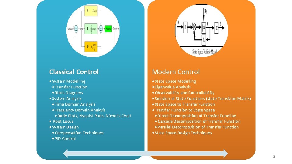
Classical Control Modern Control • System Modelling • Transfer Function • Block Diagrams • System Analysis • Time Domain Analysis • Frequency Domain Analysis • Bode Plots, Nyquist Plots, Nichol’s Chart • Root Locus • System Design • Compensation Techniques • PID Control • State Space Modelling • Eigenvalue Analysis • Observability and Controllability • Solution of State Equations (state Transition Matrix) • State Space to Transfer Function • Transfer Function to State Space • Direct Decomposition of Transfer Function • Cascade Decomposition of Transfer Function • Parallel Decomposition of Transfer Function • State Space Design Techniques 3

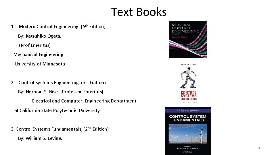
Text Books 1. Modern Control Engineering, (5 th Edition) By: Katsuhiko Ogata. (Prof Emeritus) Mechanical Engineering University of Minnesota 2. Control Systems Engineering, (6 th Edition) By: Norman S. Nise. (Professor Emeritus) Electrical and Computer Engineering Department at California State Polytechnic University 3. Control Systems Fundamentals, (2 nd Edition) By: William S. Levine. 4

Reference Books 1. Modern Control Systems, (12 th Edition) By: Richard C. Dorf and Robert H. Bishop. 2. Automatic Control Systems, (9 th Edition) By: Golnaraghi and B. C. Kuo. 5

Prerequisites • For Classical Control Theory – Differential Equations – Laplace Transform – Basic Physics – Ordinary and Semi-logarithimic graph papers 6

Introduction to Control Systems A control system consisting of interconnected components is designed to achieve a desired purpose. To understand the purpose of a control system, it is useful to examine examples of control systems through the course of history. These early systems incorporated many of the same ideas of feedback that are in use today. Modern control engineering practice includes the use of control design strategies for improving manufacturing processes, the efficiency of energy use, advanced automobile control, including rapid transit, among others.

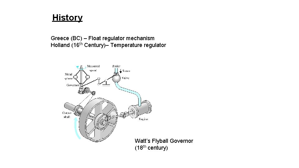
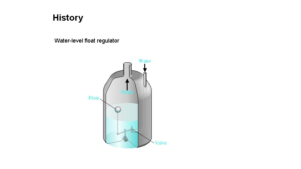
History Greece (BC) – Float regulator mechanism Holland (16 th Century)– Temperature regulator Watt’s Flyball Governor (18 th century)

History Water-level float regulator

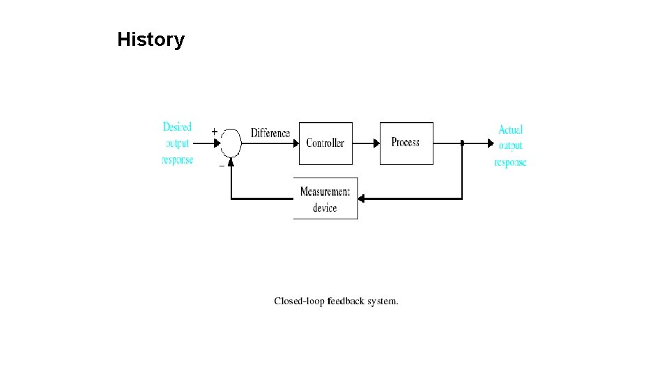
History

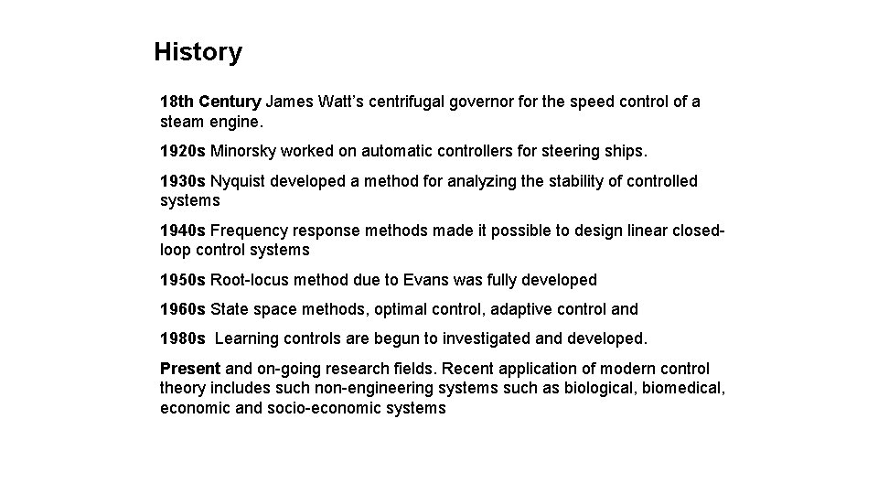
History 18 th Century James Watt’s centrifugal governor for the speed control of a steam engine. 1920 s Minorsky worked on automatic controllers for steering ships. 1930 s Nyquist developed a method for analyzing the stability of controlled systems 1940 s Frequency response methods made it possible to design linear closedloop control systems 1950 s Root-locus method due to Evans was fully developed 1960 s State space methods, optimal control, adaptive control and 1980 s Learning controls are begun to investigated and developed. Present and on-going research fields. Recent application of modern control theory includes such non-engineering systems such as biological, biomedical, economic and socio-economic systems

What is Control System? • A system Controlling the operation of another system. • A system that can regulate itself and another system. • A control System is a device, or set of devices to manage, command, direct or regulate the behaviour of other device(s) or system(s). 12

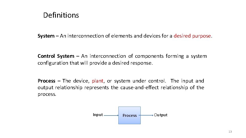
Definitions System – An interconnection of elements and devices for a desired purpose. Control System – An interconnection of components forming a system configuration that will provide a desired response. Process – The device, plant, or system under control. The input and output relationship represents the cause-and-effect relationship of the process. Input Process Output 13

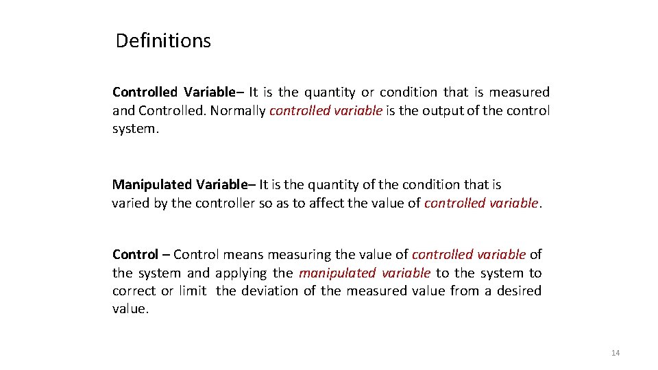
Definitions Controlled Variable– It is the quantity or condition that is measured and Controlled. Normally controlled variable is the output of the control system. Manipulated Variable– It is the quantity of the condition that is varied by the controller so as to affect the value of controlled variable. Control – Control means measuring the value of controlled variable of the system and applying the manipulated variable to the system to correct or limit the deviation of the measured value from a desired value. 14

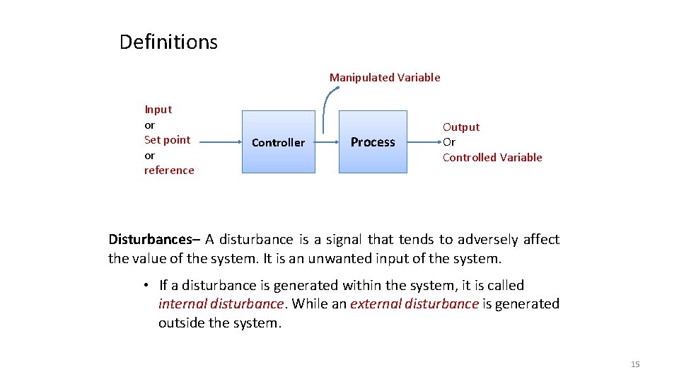
Definitions Manipulated Variable Input or Set point or reference Controller Process Output Or Controlled Variable Disturbances– A disturbance is a signal that tends to adversely affect the value of the system. It is an unwanted input of the system. • If a disturbance is generated within the system, it is called internal disturbance. While an external disturbance is generated outside the system. 15

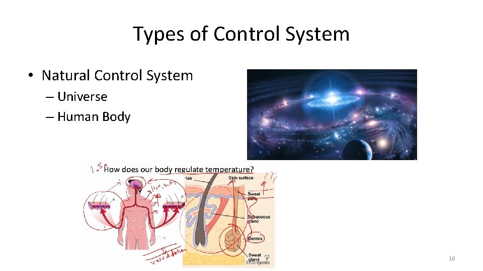
Types of Control System • Natural Control System – Universe – Human Body 16

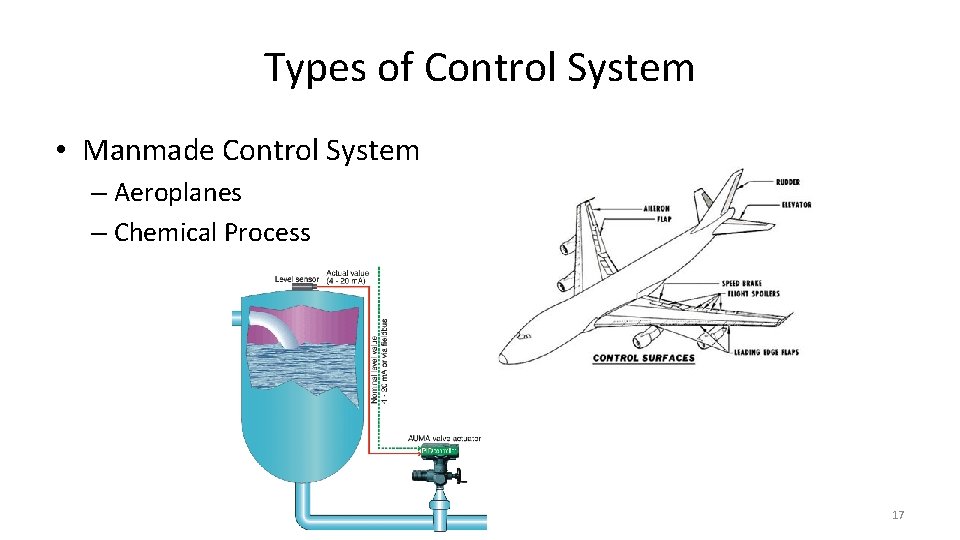
Types of Control System • Manmade Control System – Aeroplanes – Chemical Process 17

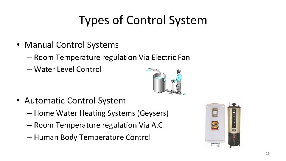
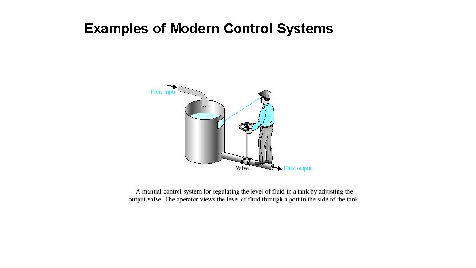
Types of Control System • Manual Control Systems – Room Temperature regulation Via Electric Fan – Water Level Control • Automatic Control System – Home Water Heating Systems (Geysers) – Room Temperature regulation Via A. C – Human Body Temperature Control 18

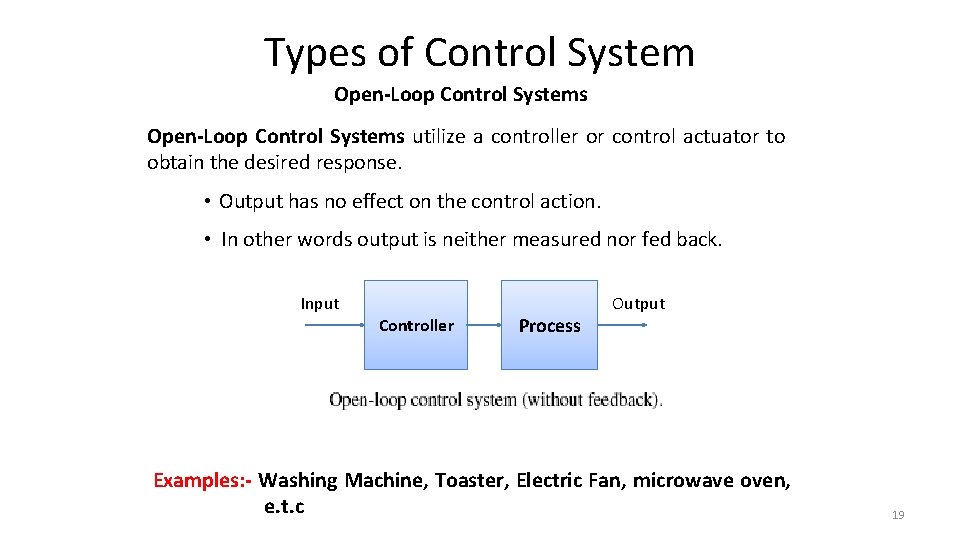
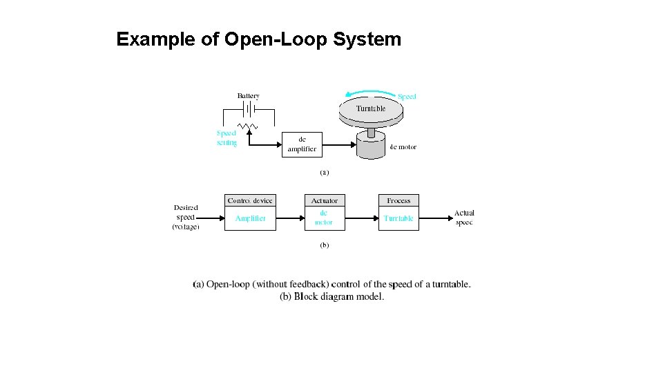
Types of Control System Open-Loop Control Systems utilize a controller or control actuator to obtain the desired response. • Output has no effect on the control action. • In other words output is neither measured nor fed back. Input Controller Process Output Examples: - Washing Machine, Toaster, Electric Fan, microwave oven, e. t. c 19

Types of Control System Open-Loop Control Systems • Since in open loop control systems reference input is not compared with measured output, for each reference input there is fixed operating condition. Therefore, the accuracy of the system depends on calibration. • The performance of open loop system is severely affected by the presence of disturbances, or variation in operating/ environmental conditions. 20

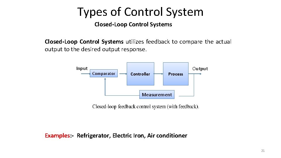
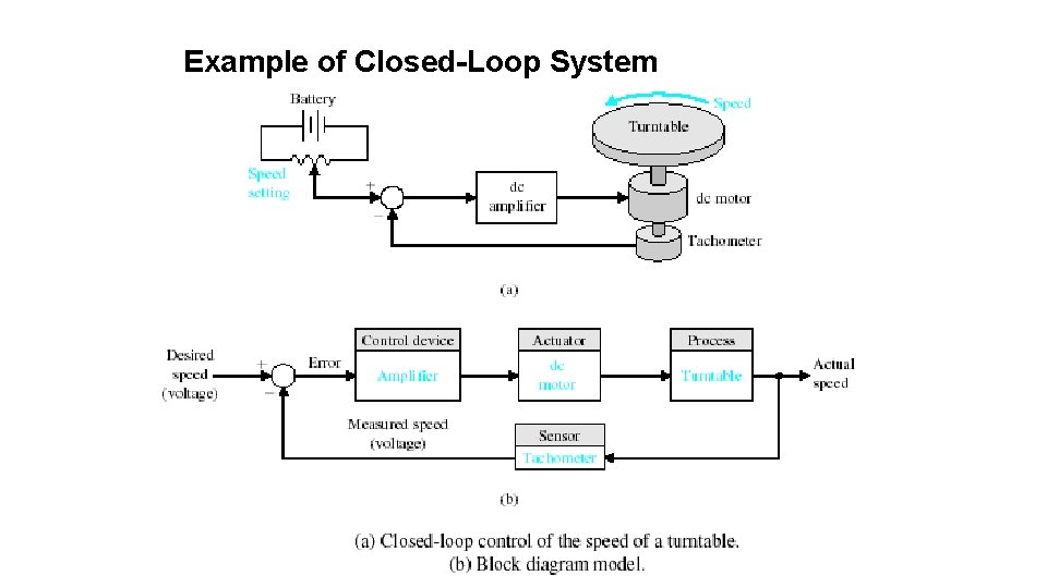
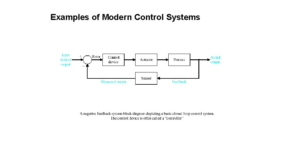
Types of Control System Closed-Loop Control Systems utilizes feedback to compare the actual output to the desired output response. Input Comparator Controller Process Output Measurement Examples: - Refrigerator, Electric Iron, Air conditioner 21

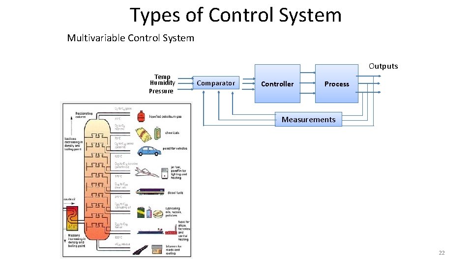
Types of Control System Multivariable Control System Outputs Temp Humidity Pressure Comparator Controller Process Measurements 22

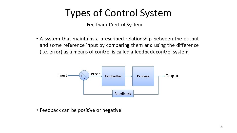
Types of Control System Feedback Control System • A system that maintains a prescribed relationship between the output and some reference input by comparing them and using the difference (i. e. error) as a means of control is called a feedback control system. Input + - error Controller Process Output Feedback • Feedback can be positive or negative. 23

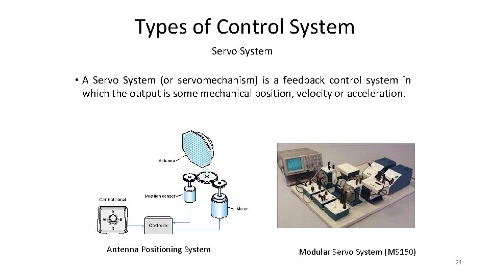
Types of Control System Servo System • A Servo System (or servomechanism) is a feedback control system in which the output is some mechanical position, velocity or acceleration. Antenna Positioning System Modular Servo System (MS 150) 24

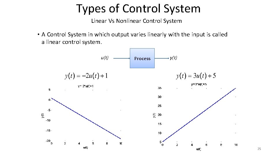
Types of Control System Linear Vs Nonlinear Control System • A Control System in which output varies linearly with the input is called a linear control system. u(t) Process y(t) 25

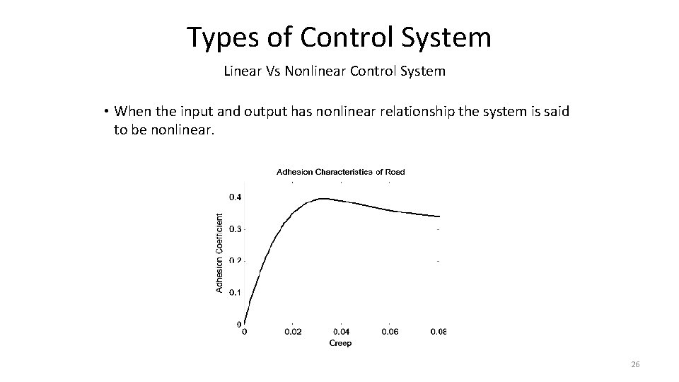
Types of Control System Linear Vs Nonlinear Control System • When the input and output has nonlinear relationship the system is said to be nonlinear. 26

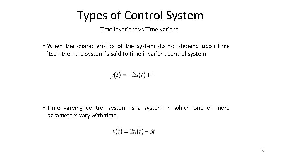
Types of Control System Time invariant vs Time variant • When the characteristics of the system do not depend upon time itself then the system is said to time invariant control system. • Time varying control system is a system in which one or more parameters vary with time. 27

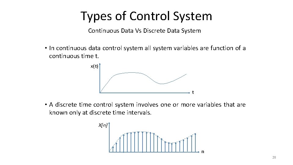
Types of Control System Continuous Data Vs Discrete Data System • In continuous data control system all system variables are function of a continuous time t. x(t) t • A discrete time control system involves one or more variables that are known only at discrete time intervals. X[n] n 28

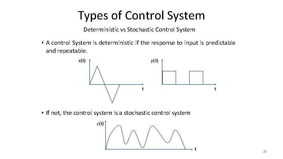
Types of Control System Deterministic vs Stochastic Control System • A control System is deterministic if the response to input is predictable and repeatable. x(t) y(t) t t • If not, the control system is a stochastic control system z(t) t 29

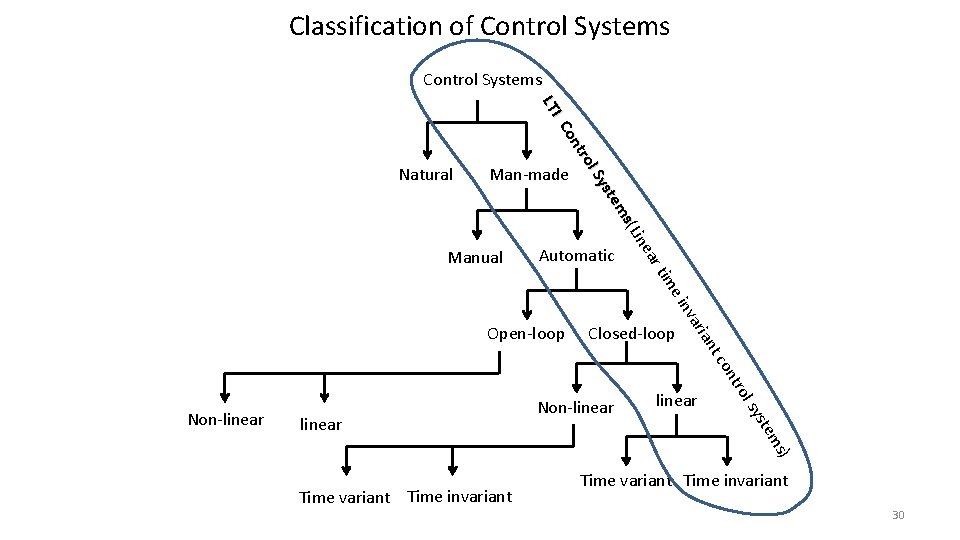
Classification of Control Systems a ine s(L em yst l. S tro on IC LT Natural Man-made Automatic rt Manual e im linear s) tem sys Non-linear l tro on linear Closed-loop tc an Non-linear ari inv Open-loop Time variant Time invariant 30

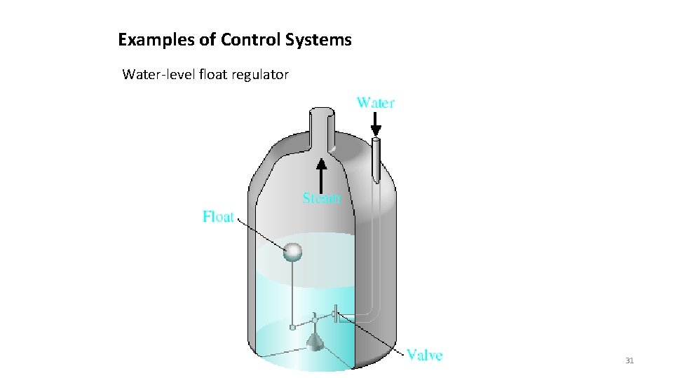
Examples of Control Systems Water-level float regulator 31

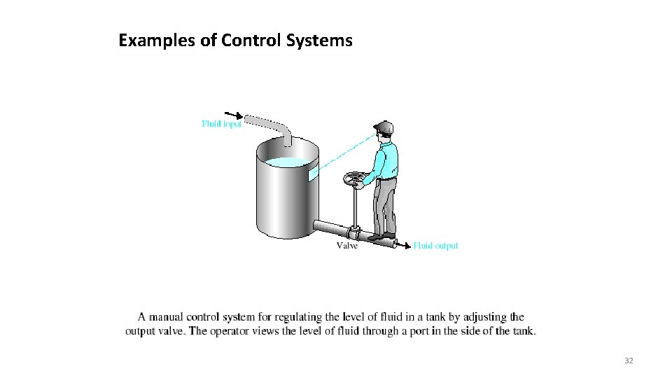
Examples of Control Systems 32

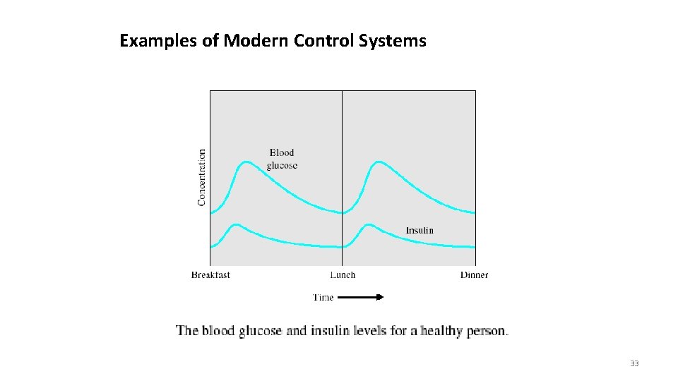
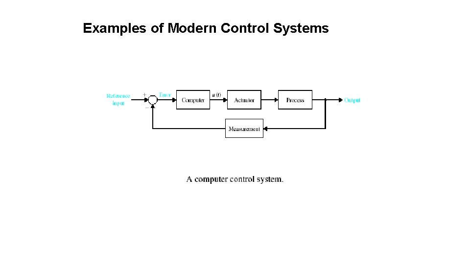
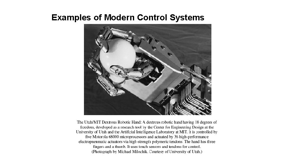
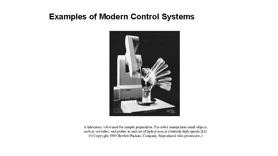
Examples of Modern Control Systems 33

Example of Open-Loop System

Example of Closed-Loop System

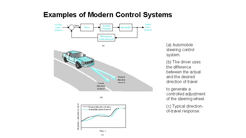
Examples of Modern Control Systems (a) Automobile steering control system. (b) The driver uses the difference between the actual and the desired direction of travel to generate a controlled adjustment of the steering wheel. (c) Typical directionof-travel response.

Examples of Modern Control Systems

Examples of Modern Control Systems

Examples of Modern Control Systems

Examples of Modern Control Systems

Examples of Modern Control Systems

Examples of Modern Control Systems

Examples of Modern Control Systems

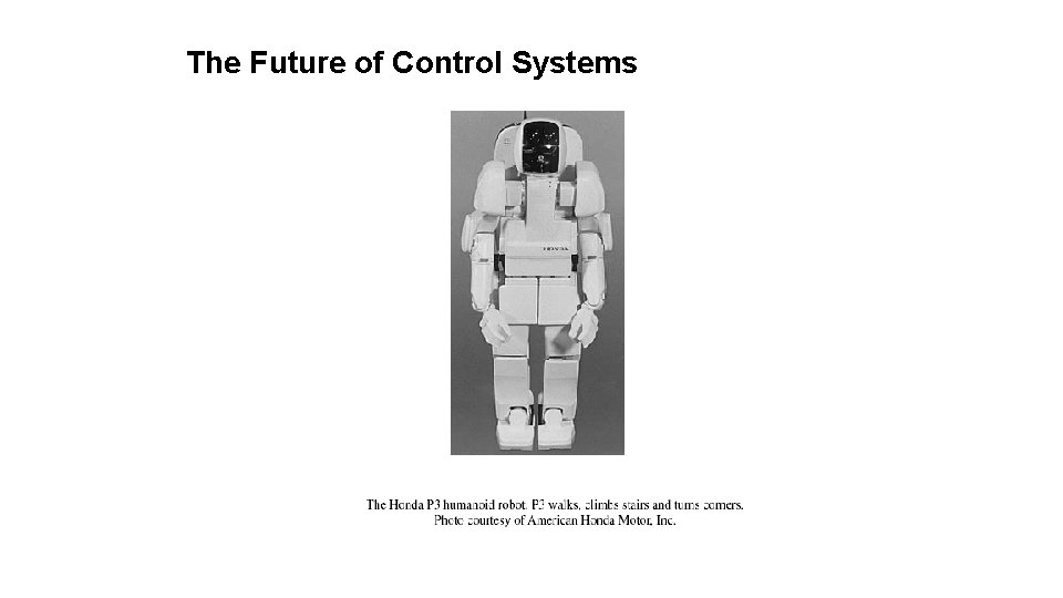
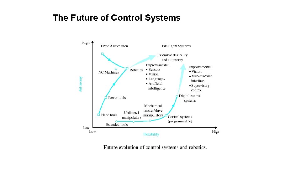
The Future of Control Systems

The Future of Control Systems

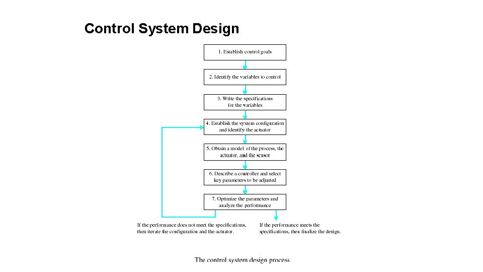
Control System Design

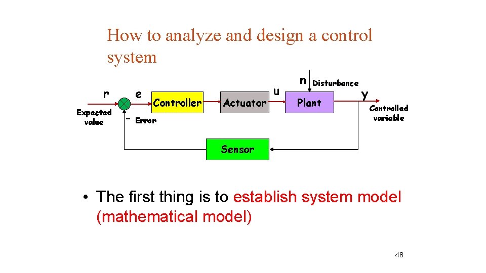
How to analyze and design a control system r Expected value e - Controller Actuator Error u n Disturbance Plant y Controlled variable Sensor • The first thing is to establish system model (mathematical model) 48

Mathematical modeling of Dynamic Systems 49

Mathematical Models of Systems Objectives We use quantitative mathematical models of physical systems to design and analyze control systems. The dynamic behavior is generally described by ordinary differential equations. We will consider a wide range of systems, including mechanical, hydraulic, and electrical. Since most physical systems are nonlinear, we will assume they are linear systems, which allow us to use Laplace transform methods. We will then proceed to obtain the input–output relationship for components and subsystems in the form of transfer functions. The transfer function blocks can be organized into block diagrams or signalflow graphs to graphically depict the interconnections. Block diagrams (and signal-flow graphs) are very convenient and natural tools for designing and analyzing complicated control systems.

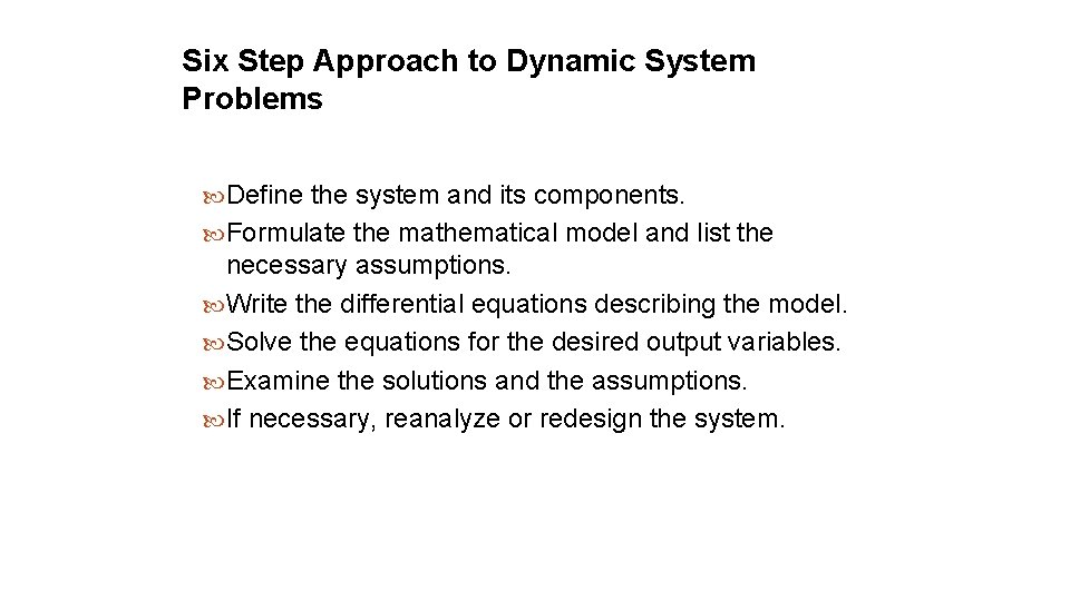
Six Step Approach to Dynamic System Problems Define the system and its components. Formulate the mathematical model and list the necessary assumptions. Write the differential equations describing the model. Solve the equations for the desired output variables. Examine the solutions and the assumptions. If necessary, reanalyze or redesign the system.

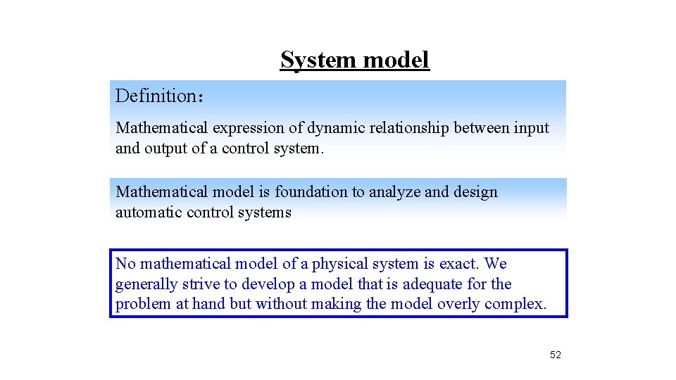
System model Definition： Mathematical expression of dynamic relationship between input and output of a control system. Mathematical model is foundation to analyze and design automatic control systems No mathematical model of a physical system is exact. We generally strive to develop a model that is adequate for the problem at hand but without making the model overly complex. 52

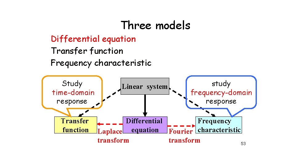
Three models Differential equation Transfer function Frequency characteristic Study time-domain response Transfer function Linear system study frequency-domain response Differential Frequency Laplace equation Fourier characteristic transform 53

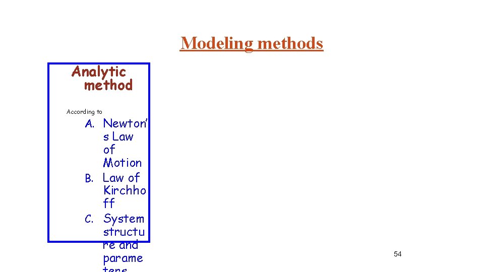
Modeling methods Analytic method According to A. Newton’ s Law of Motion B. Law of Kirchho ff C. System structu re and parame 54

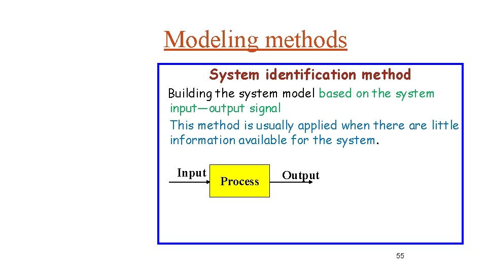
Modeling methods System identification method Building the system model based on the system input—output signal This method is usually applied when there are little information available for the system. Input Process Output 55

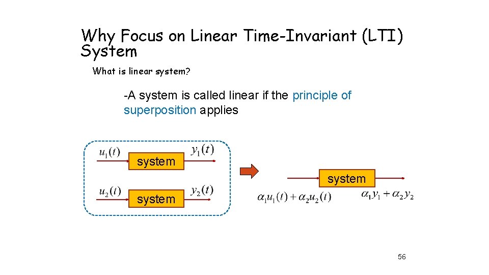
Why Focus on Linear Time-Invariant (LTI) System What is linear system? -A system is called linear if the principle of superposition applies system 56

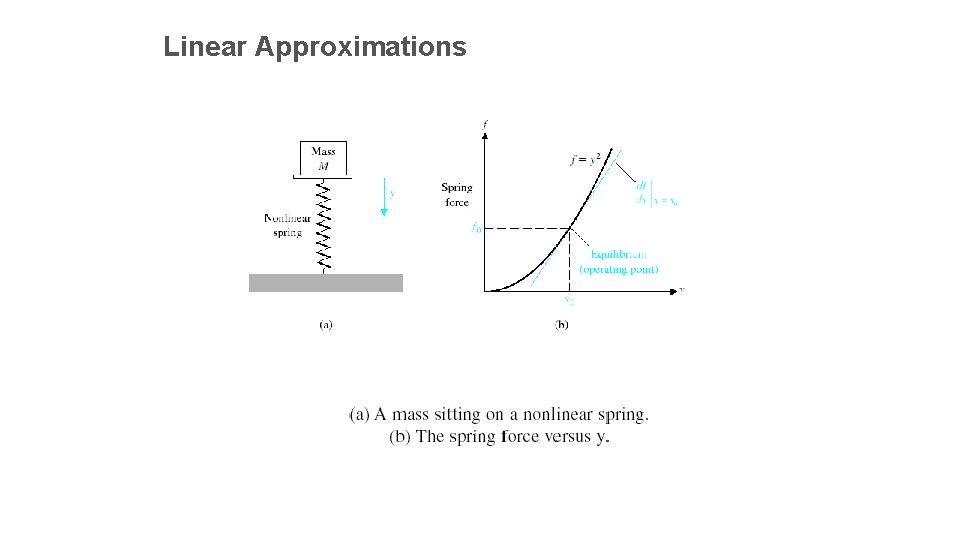
Linear Approximations

Linear Approximations Linear Systems-Necessary condition: 1. Principle of Superposition 2. Property of Homogeneity

Advantages of linear systems The overall response of a linear system can be obtained by: -- decomposing the input into a sum of elementary signals -- figuring out each response to the respective elementary signal -- adding all these responses together. Thus, we can use typical elementary signal (e. g. unit step , unit impulse, unit ramp) to analyze system for the sake of simplicity. 59

• What is time-invariant system? – A system is called time-invariant if the parameters are stationary with respect to time during system operation – Examples？ 60

Establishment of differential equation and linearization 61

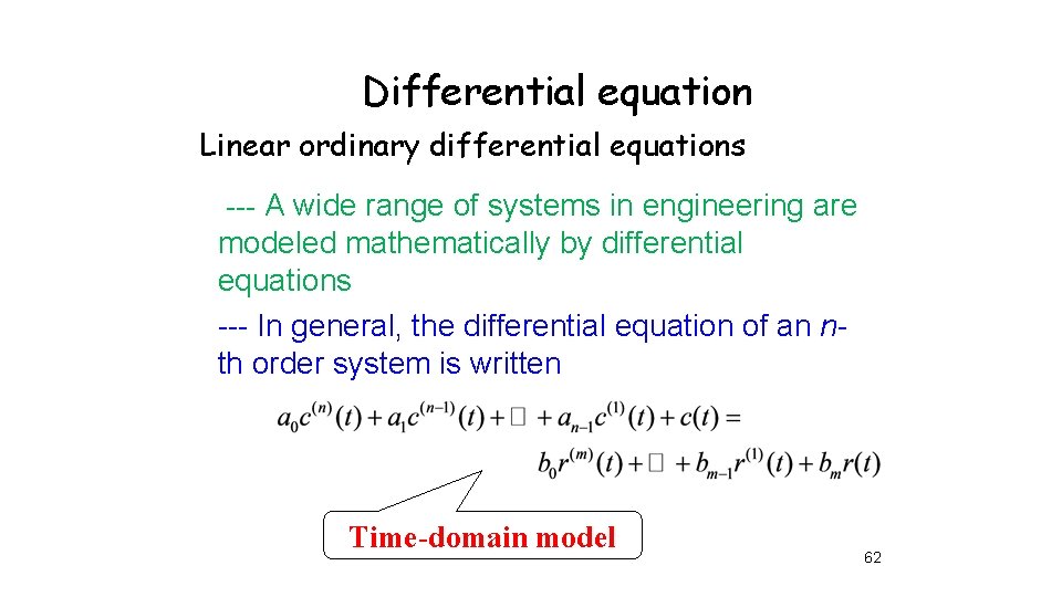
Differential equation Linear ordinary differential equations --- A wide range of systems in engineering are modeled mathematically by differential equations --- In general, the differential equation of an nth order system is written Time-domain model 62

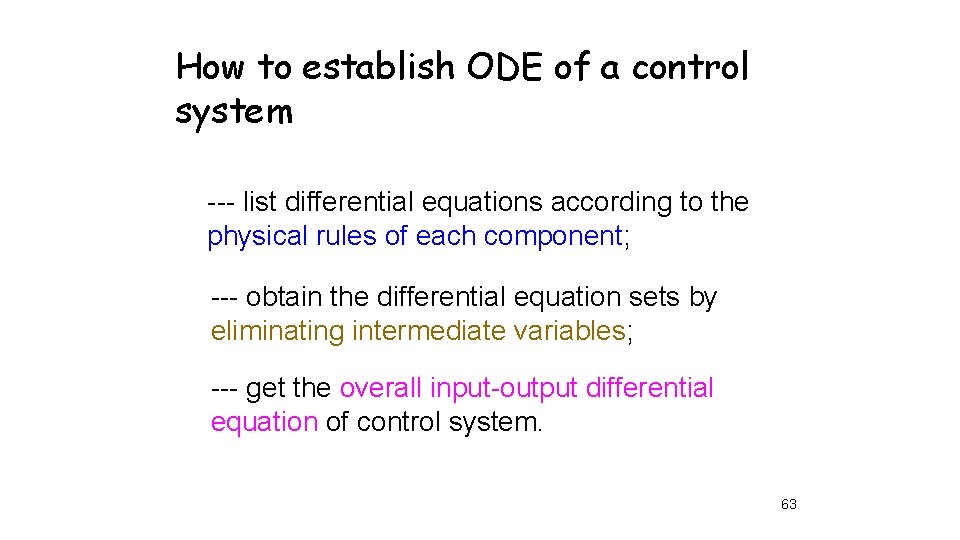
How to establish ODE of a control system --- list differential equations according to the physical rules of each component; --- obtain the differential equation sets by eliminating intermediate variables; --- get the overall input-output differential equation of control system. 63

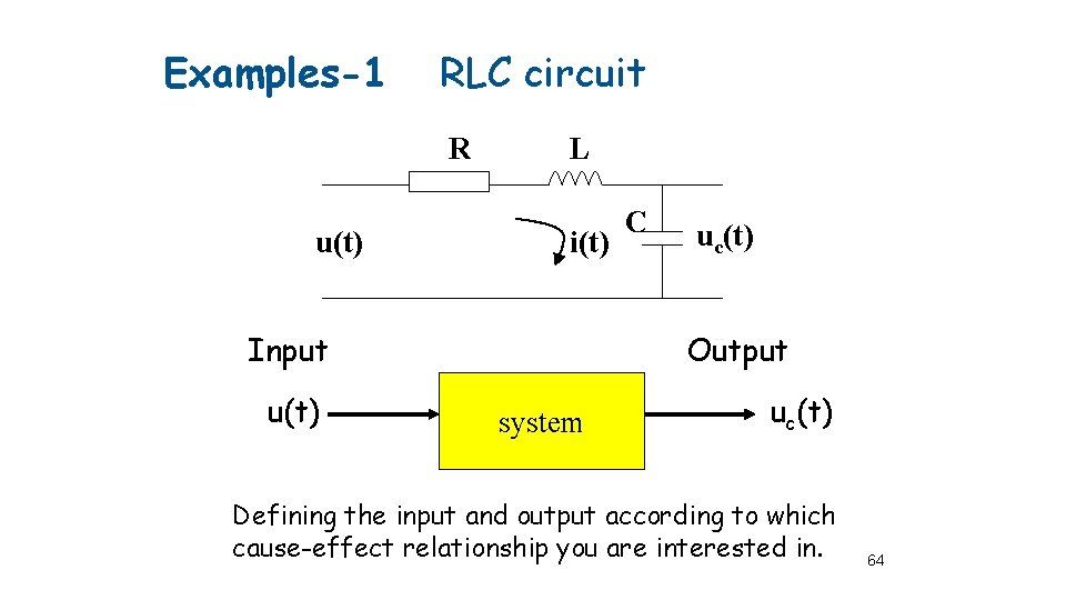
Examples-1 RLC circuit R u(t) L i(t) Input u(t) C uc(t) Output system uc(t) Defining the input and output according to which cause-effect relationship you are interested in. 64

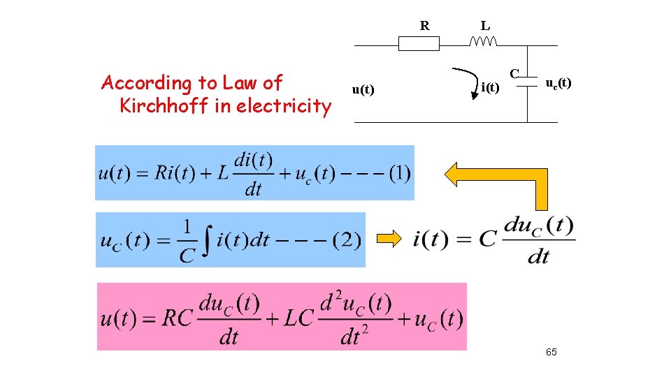
R According to Law of Kirchhoff in electricity u(t) L i(t) C uc(t) 65

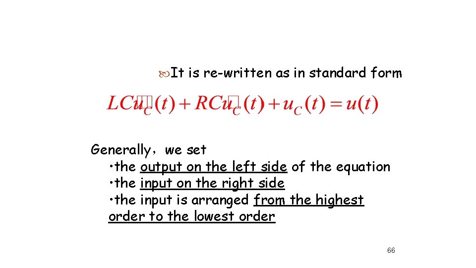
It is re-written as in standard form Generally，we set • the output on the left side of the equation • the input on the right side • the input is arranged from the highest order to the lowest order 66

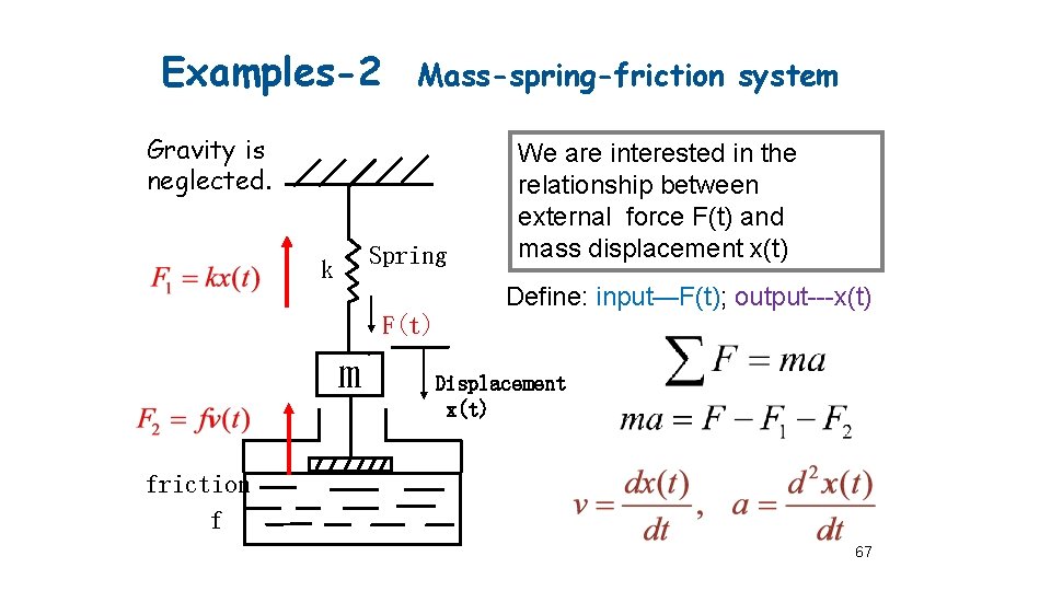
Examples-2 Mass-spring-friction system Gravity is neglected. Spring k We are interested in the relationship between external force F(t) and mass displacement x(t) Define: input—F(t); output---x(t) F(t) m Displacement x(t) friction f 67

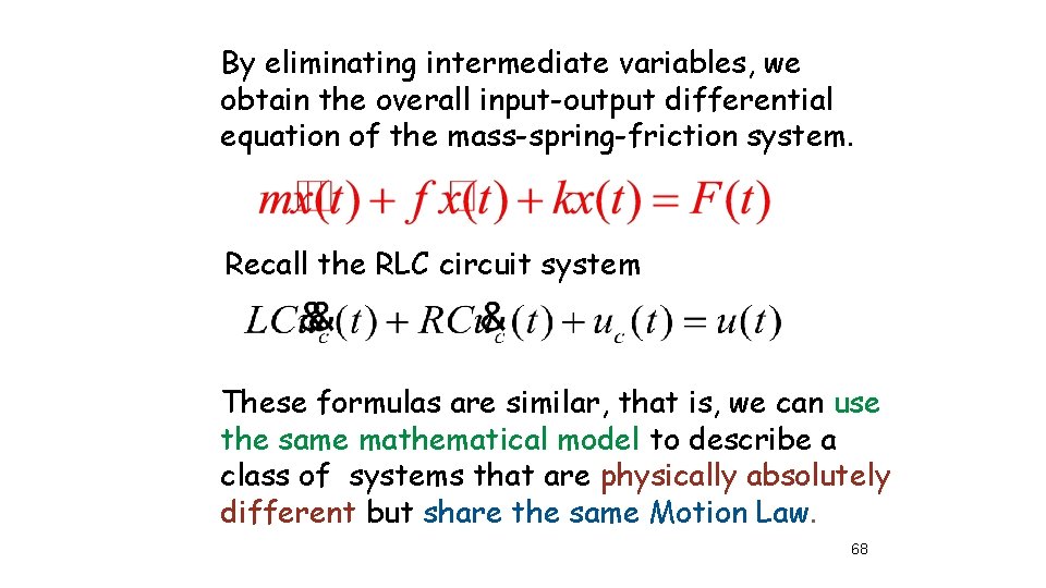
By eliminating intermediate variables, we obtain the overall input-output differential equation of the mass-spring-friction system. Recall the RLC circuit system These formulas are similar, that is, we can use the same mathematical model to describe a class of systems that are physically absolutely different but share the same Motion Law. 68

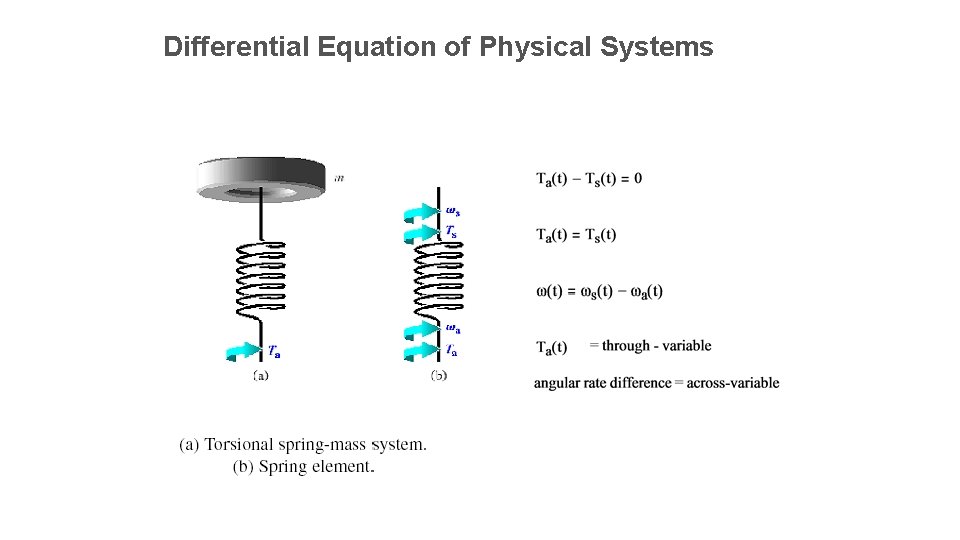
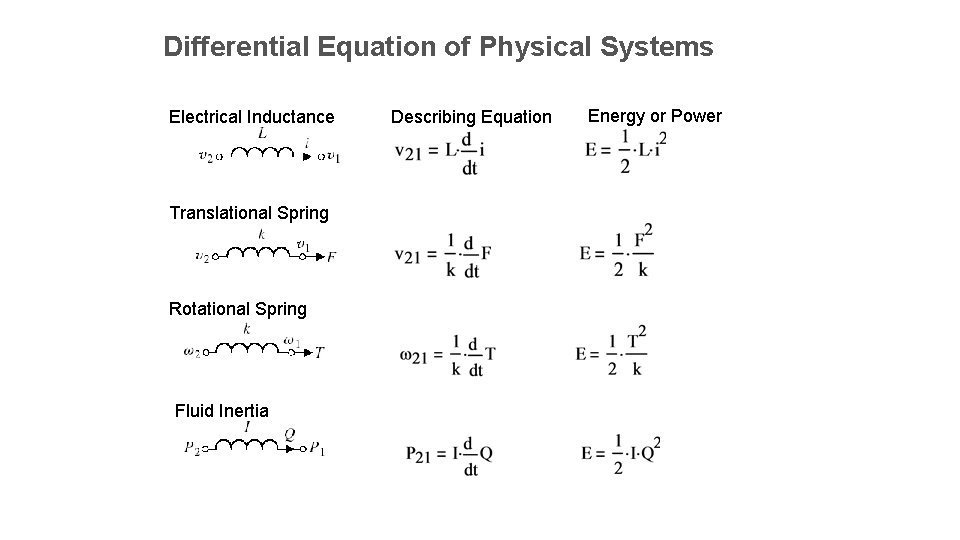
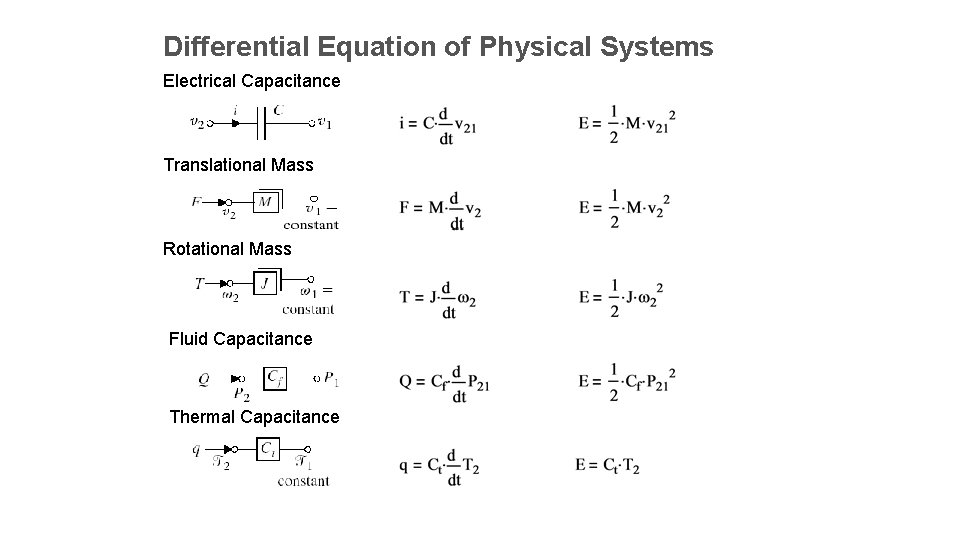
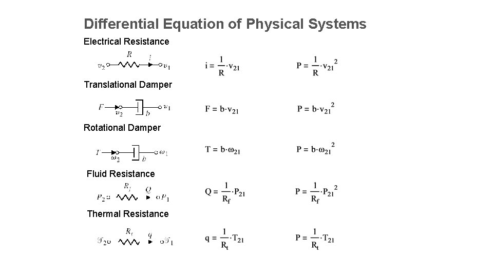
Differential Equation of Physical Systems

Differential Equation of Physical Systems Electrical Inductance Translational Spring Rotational Spring Fluid Inertia Describing Equation Energy or Power

Differential Equation of Physical Systems Electrical Capacitance Translational Mass Rotational Mass Fluid Capacitance Thermal Capacitance

Differential Equation of Physical Systems Electrical Resistance Translational Damper Rotational Damper Fluid Resistance Thermal Resistance

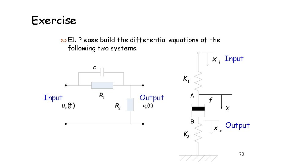
Exercise E 1. Please build the differential equations of the following two systems. Input Output A x B Output 73

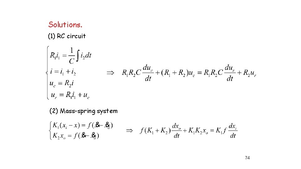
Solutions. (1) RC circuit (2) Mass-spring system 74

Transfer function 75

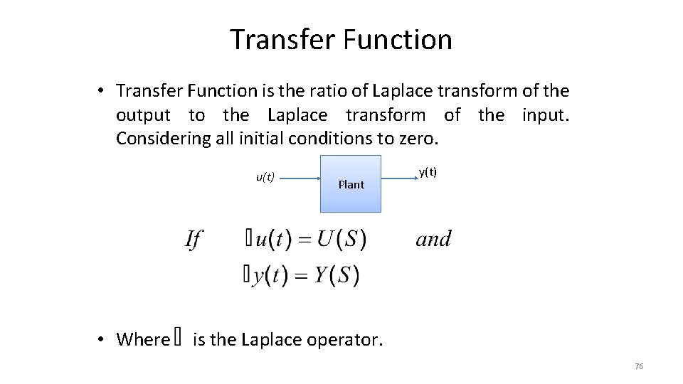
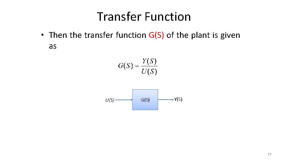
Transfer Function • Transfer Function is the ratio of Laplace transform of the output to the Laplace transform of the input. Considering all initial conditions to zero. u(t) • Where Plant y(t) is the Laplace operator. 76

Transfer Function • Then the transfer function G(S) of the plant is given as U(S) G(S) Y(S) 77

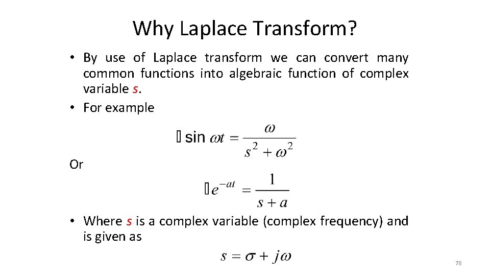
Why Laplace Transform? • By use of Laplace transform we can convert many common functions into algebraic function of complex variable s. • For example Or • Where s is a complex variable (complex frequency) and is given as 78

The Laplace Transform Historical Perspective - Heaviside’s Operators Origin of Operational Calculus (1887)

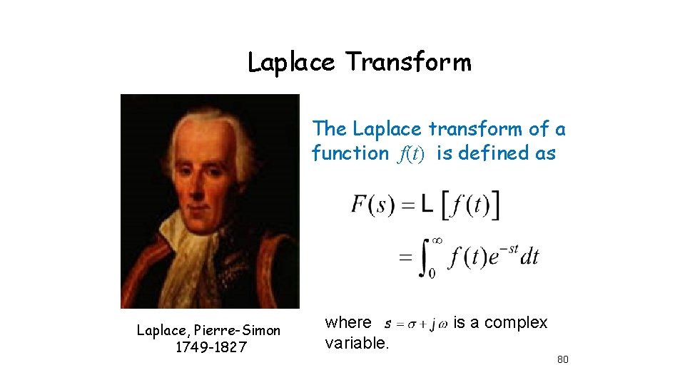
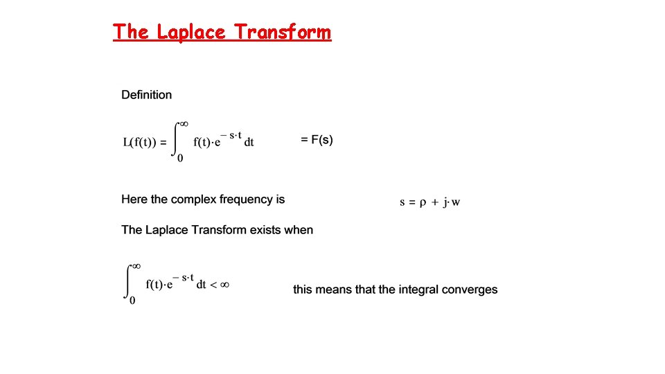
Laplace Transform The Laplace transform of a function f(t) is defined as Laplace, Pierre-Simon 1749 -1827 where variable. is a complex 80

The Laplace Transform

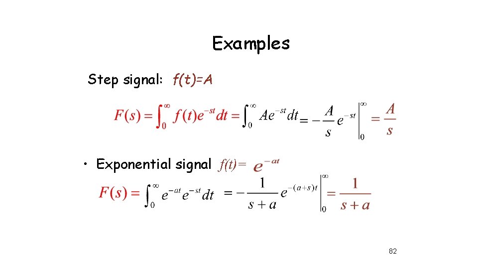
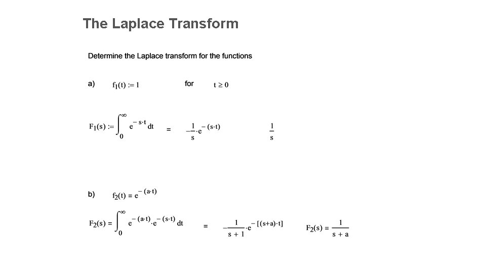
Examples Step signal: f(t)=A • Exponential signal f(t)= 82

The Laplace Transform

The Laplace Transform

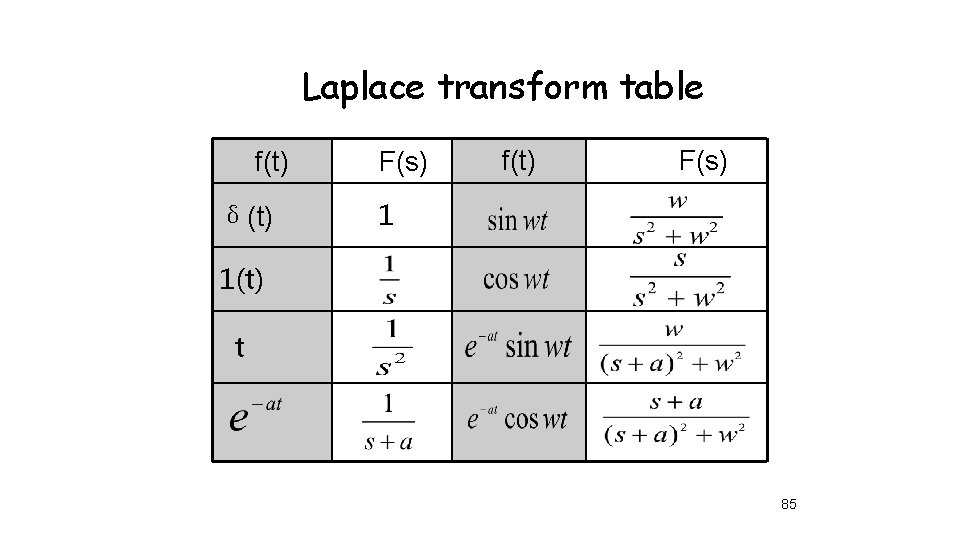
Laplace transform table f(t) δ(t) F(s) f(t) F(s) 1 1(t) t 85

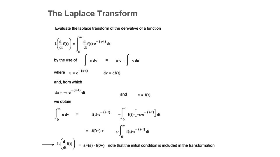
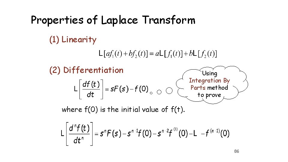
Properties of Laplace Transform (1) Linearity (2) Differentiation Using Integration By Parts method to prove where f(0) is the initial value of f(t). 86

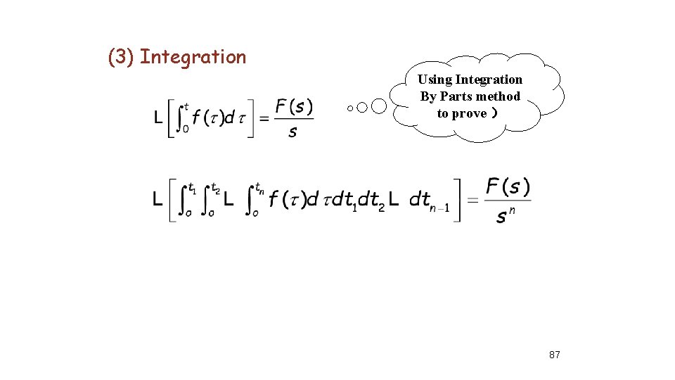
(3) Integration Using Integration By Parts method to prove ） 87

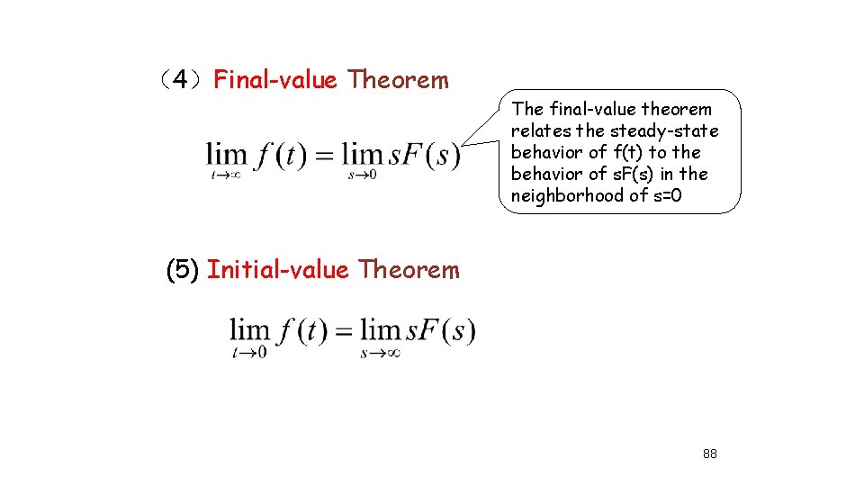
（4）Final-value Theorem The final-value theorem relates the steady-state behavior of f(t) to the behavior of s. F(s) in the neighborhood of s=0 (5) Initial-value Theorem 88

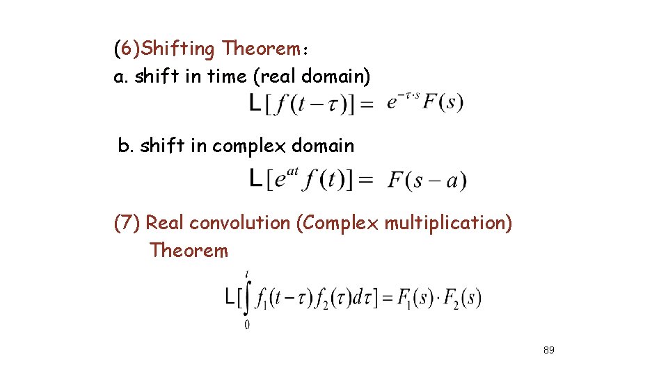
(6)Shifting Theorem： a. shift in time (real domain) b. shift in complex domain (7) Real convolution (Complex multiplication) Theorem 89

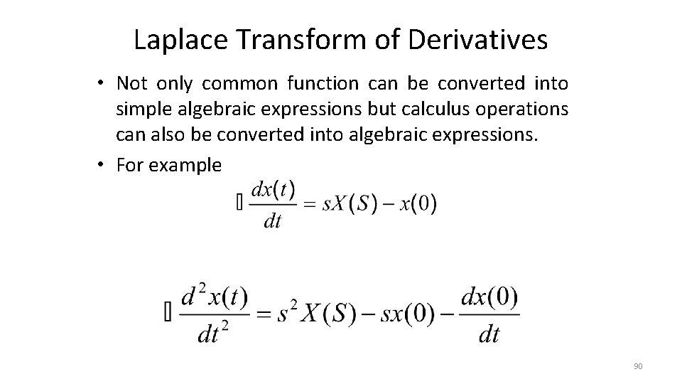
Laplace Transform of Derivatives • Not only common function can be converted into simple algebraic expressions but calculus operations can also be converted into algebraic expressions. • For example 90

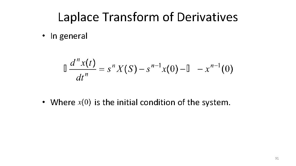
Laplace Transform of Derivatives • In general • Where is the initial condition of the system. 91

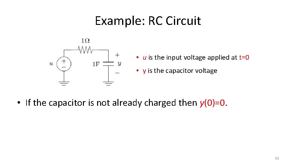
Example: RC Circuit • u is the input voltage applied at t=0 • y is the capacitor voltage • If the capacitor is not already charged then y(0)=0. 92

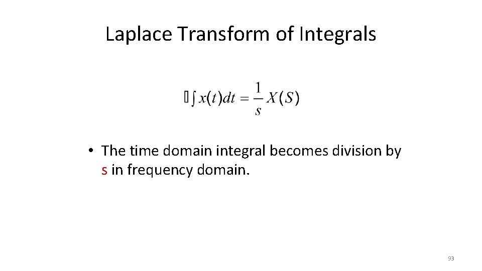
Laplace Transform of Integrals • The time domain integral becomes division by s in frequency domain. 93

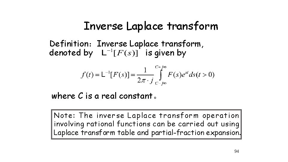
Inverse Laplace transform Definition：Inverse Laplace transform, denoted by is given by where C is a real constant。 Note: The inverse Laplace transform operation involving rational functions can be carried out using Laplace transform table and partial-fraction expansion. 94

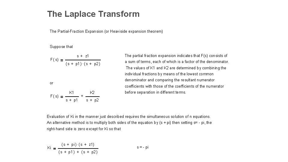
The Laplace Transform The Partial-Fraction Expansion (or Heaviside expansion theorem) Suppose that F( s) s + z 1 The partial fraction expansion indicates that F(s) consists of ( s + p 1 ) × ( s + p 2 ) a sum of terms, each of which is a factor of the denominator. The values of K 1 and K 2 are determined by combining the individual fractions by means of the lowest common denominator and comparing the resultant numerator or coefficients with those of the coefficients of the numerator F( s) K 1 s + p 1 + K 2 before separation in different terms. s + p 2 Evaluation of Ki in the manner just described requires the simultaneous solution of n equations. An alternative method is to multiply both sides of the equation by (s + pi) then setting s= - pi, the right-hand side is zero except for Ki so that Ki ( s + pi ) × ( s + z 1) ( s + p 1 ) + ( s + p 2 ) s = - pi

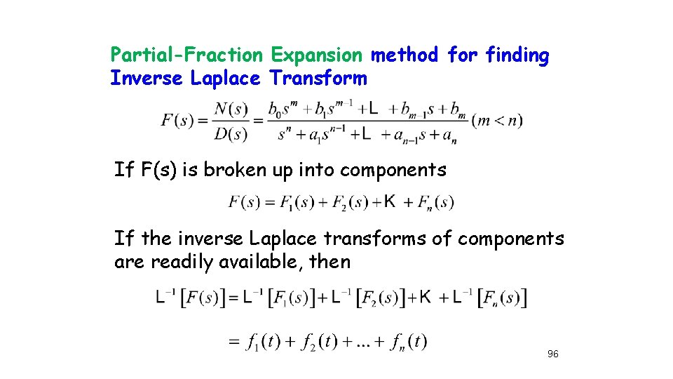
Partial-Fraction Expansion method for finding Inverse Laplace Transform If F(s) is broken up into components If the inverse Laplace transforms of components are readily available, then 96

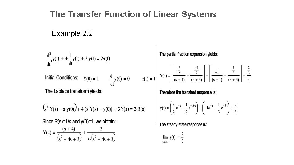
The Transfer Function of Linear Systems Example 2. 2

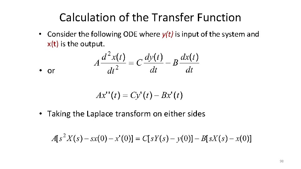
Calculation of the Transfer Function • Consider the following ODE where y(t) is input of the system and x(t) is the output. • or • Taking the Laplace transform on either sides 98

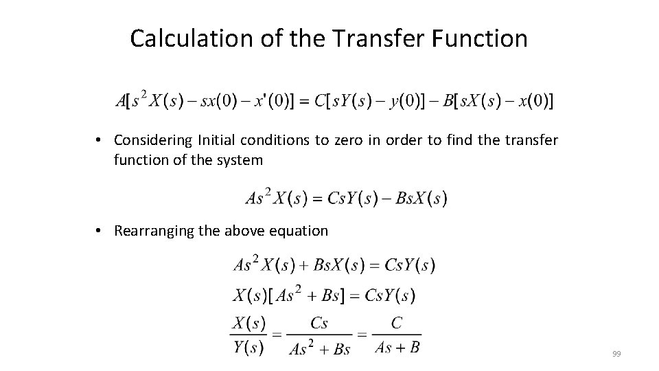
Calculation of the Transfer Function • Considering Initial conditions to zero in order to find the transfer function of the system • Rearranging the above equation 99

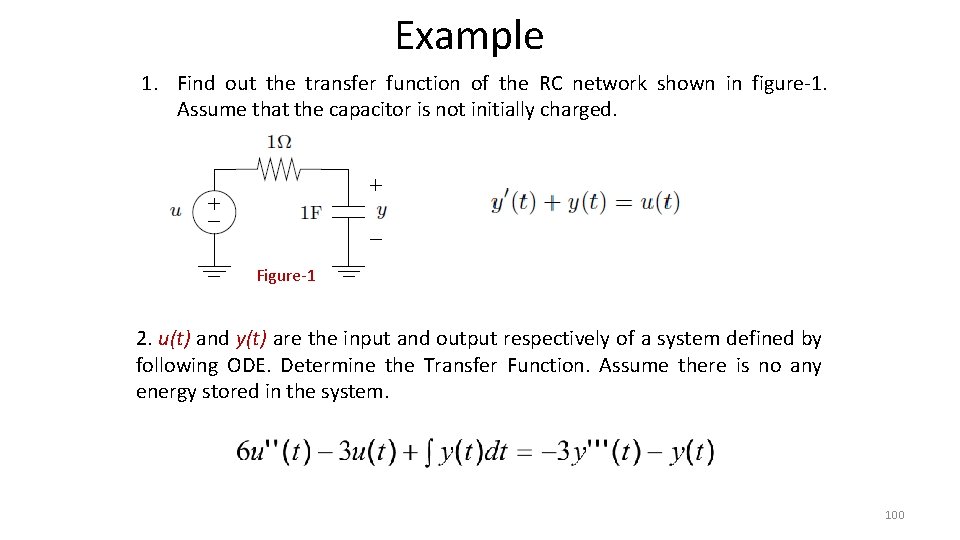
Example 1. Find out the transfer function of the RC network shown in figure-1. Assume that the capacitor is not initially charged. Figure-1 2. u(t) and y(t) are the input and output respectively of a system defined by following ODE. Determine the Transfer Function. Assume there is no any energy stored in the system. 100

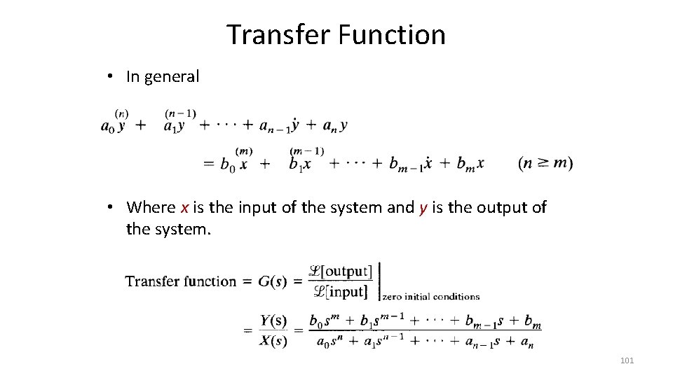
Transfer Function • In general • Where x is the input of the system and y is the output of the system. 101

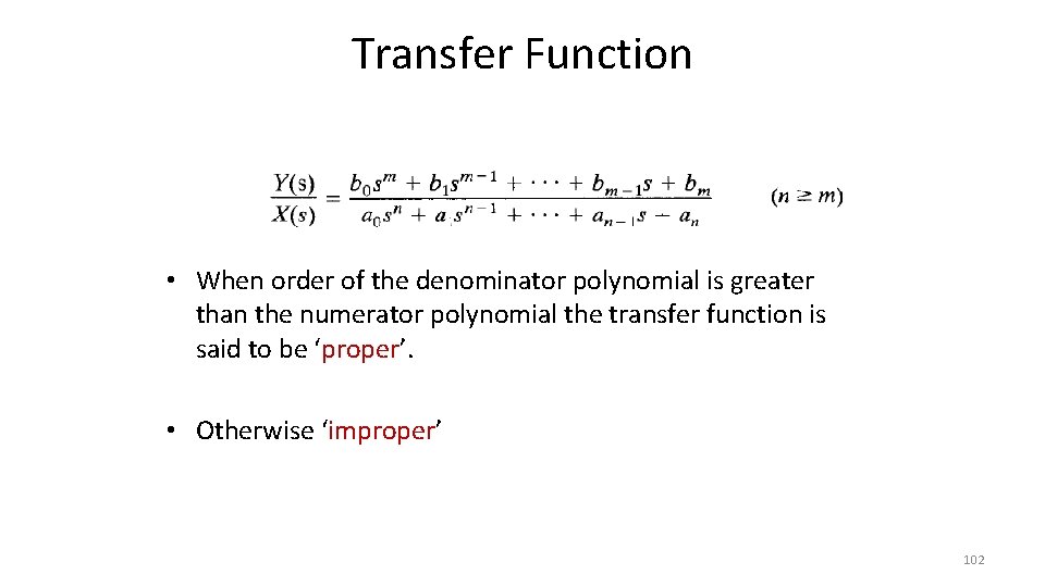
Transfer Function • When order of the denominator polynomial is greater than the numerator polynomial the transfer function is said to be ‘proper’. • Otherwise ‘improper’ 102

Transfer Function • Transfer function helps us to check – The stability of the system – Time domain and frequency domain characteristics of the system – Response of the system for any given input 103

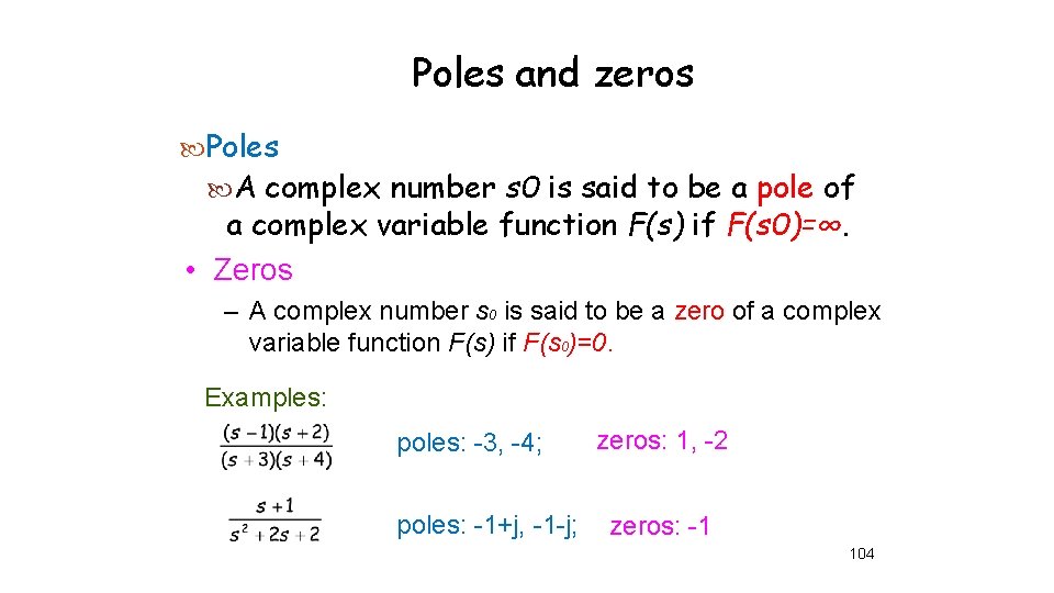
Poles and zeros Poles A complex number s 0 is said to be a pole of a complex variable function F(s) if F(s 0)=∞. • Zeros – A complex number s 0 is said to be a zero of a complex variable function F(s) if F(s 0)=0. Examples: poles: -3, -4; poles: -1+j, -1 -j; zeros: 1, -2 zeros: -1 104

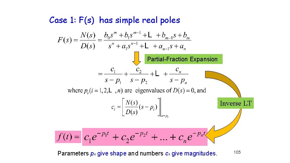
Case 1: F(s) has simple real poles Partial-Fraction Expansion Inverse LT Parameters pk give shape and numbers ck give magnitudes. 105

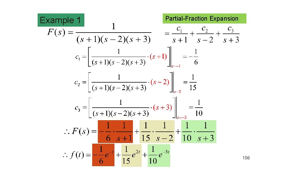
Example 1 Partial-Fraction Expansion 106

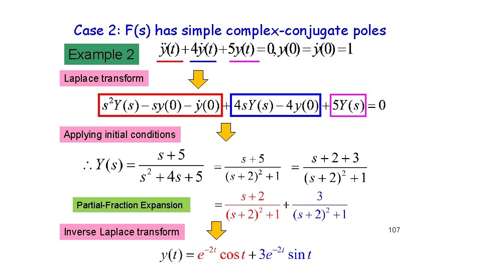
Case 2: F(s) has simple complex-conjugate poles Example 2 Laplace transform Applying initial conditions Partial-Fraction Expansion Inverse Laplace transform 107

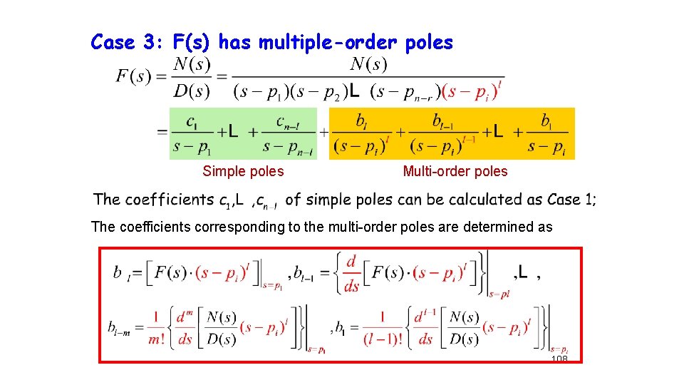
Case 3: F(s) has multiple-order poles Simple poles Multi-order poles The coefficients corresponding to the multi-order poles are determined as 108

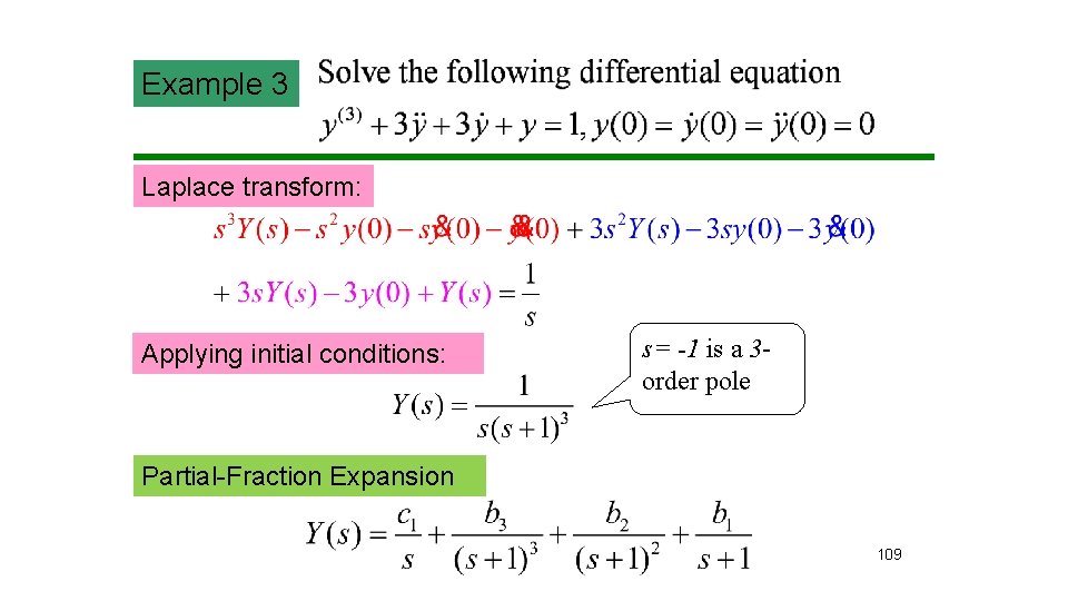
Example 3 Laplace transform: Applying initial conditions: s= -1 is a 3 order pole Partial-Fraction Expansion 109

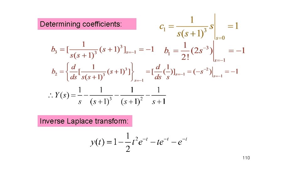
Determining coefficients: Inverse Laplace transform: 110

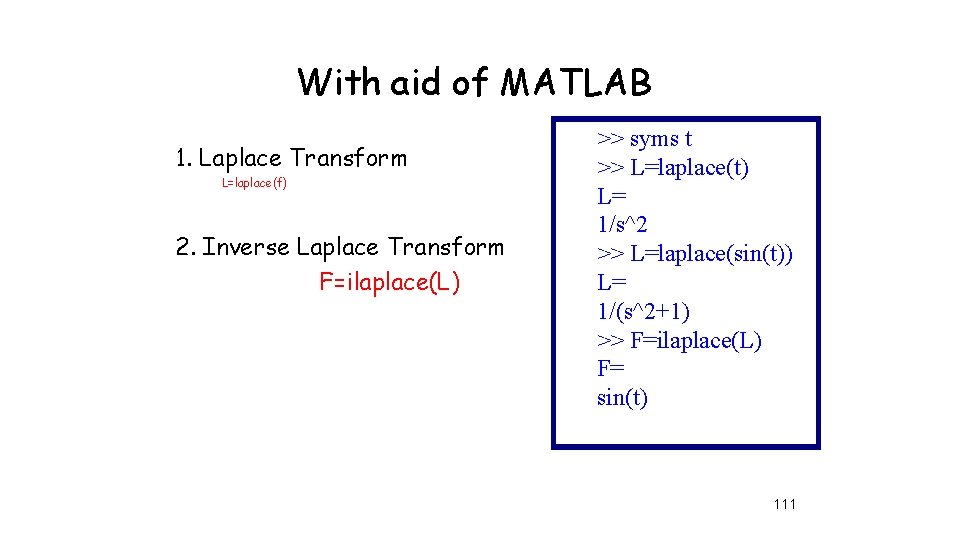
With aid of MATLAB 1. Laplace Transform L=laplace(f) 2. Inverse Laplace Transform F=ilaplace(L) >> syms t >> L=laplace(t) L= 1/s^2 >> L=laplace(sin(t)) L= 1/(s^2+1) >> F=ilaplace(L) F= sin(t) 111

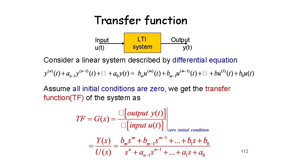
Transfer function Input u(t) LTI system Output y(t) Consider a linear system described by differential equation Assume all initial conditions are zero, we get the transfer function(TF) of the system as 112

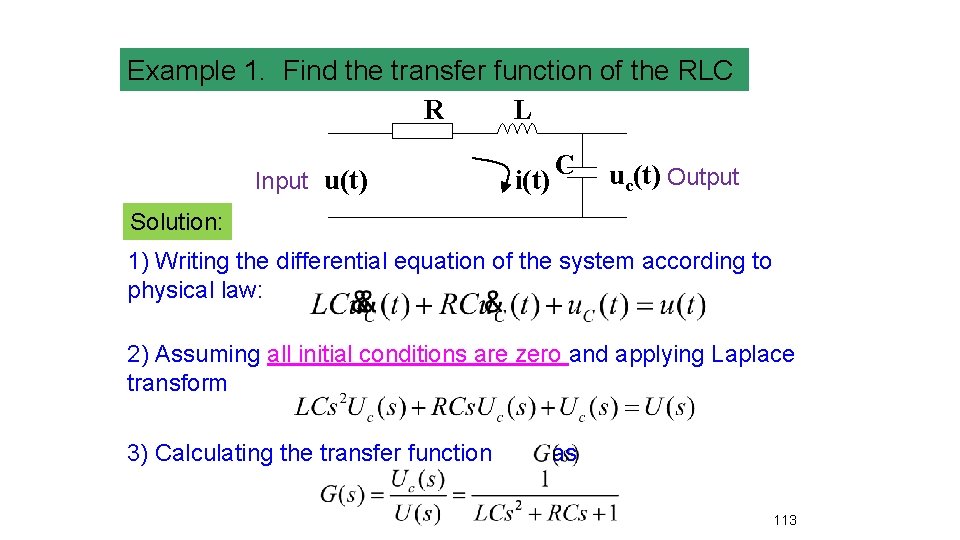
Example 1. Find the transfer function of the RLC R L Input u(t) i(t) C uc(t) Output Solution: 1) Writing the differential equation of the system according to physical law: 2) Assuming all initial conditions are zero and applying Laplace transform 3) Calculating the transfer function as 113

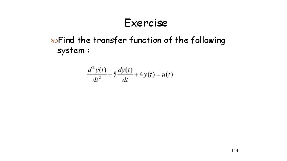
Exercise Find the transfer function of the following system : 114

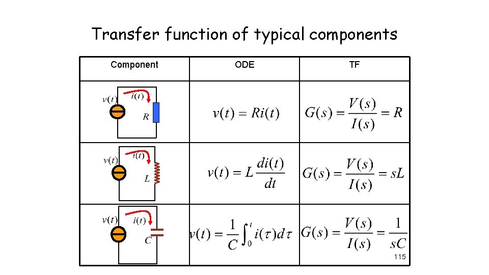
Transfer function of typical components Component ODE TF 115

Properties of transfer function The transfer function is defined only for a linear time-invariant system, not for nonlinear system. All initial conditions of the system are set to zero. The transfer function is independent of the input of the system. The transfer function G(s) is the Laplace transform of the unit impulse response g(t). 116

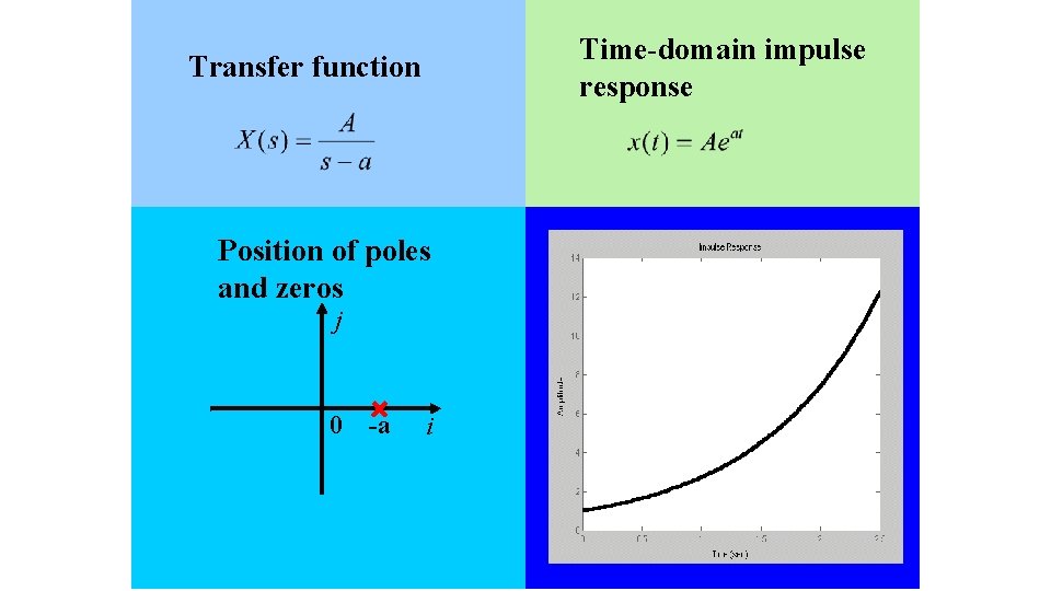
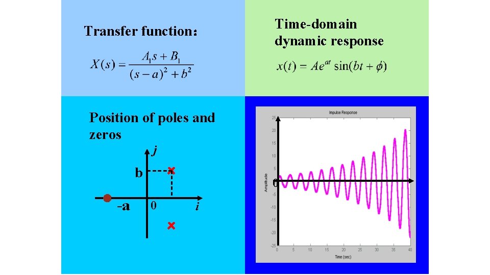
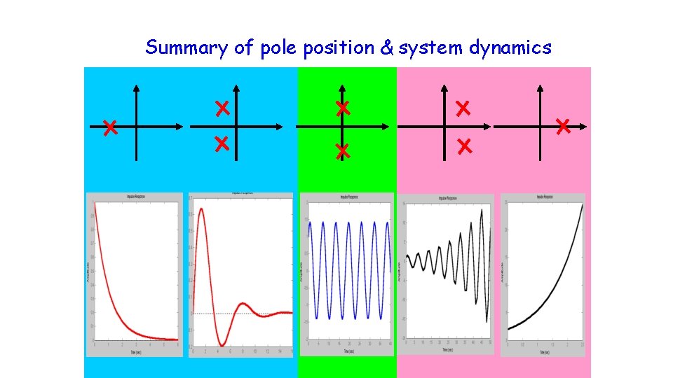
How poles and zeros relate to system response • Why we strive to obtain TF models? • Why control engineers prefer to use TF model? • How to use TF model to analyze and design control systems? • we start from the relationship between the locations of zeros and poles of TF and the output responses of a system 117

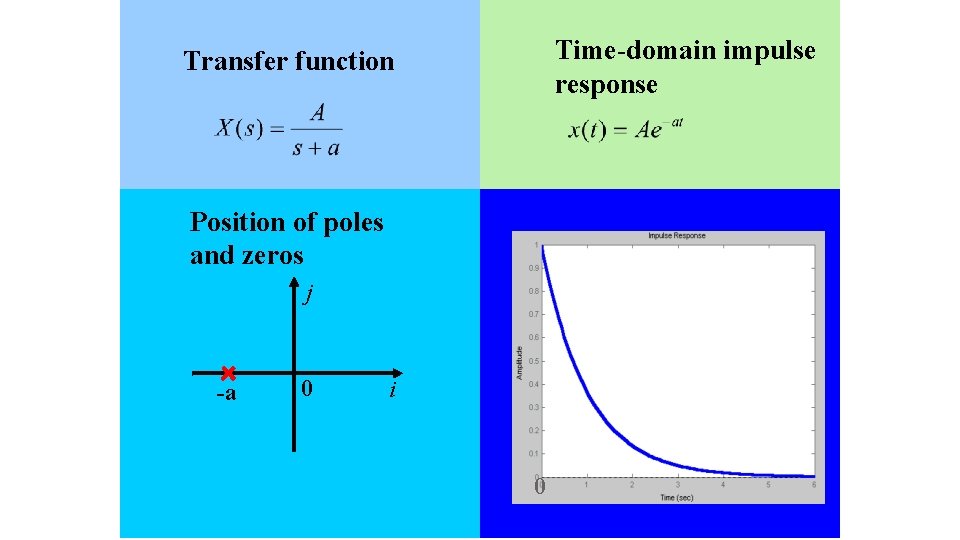
Time-domain impulse response Transfer function Position of poles and zeros j -a 0 i 0 118

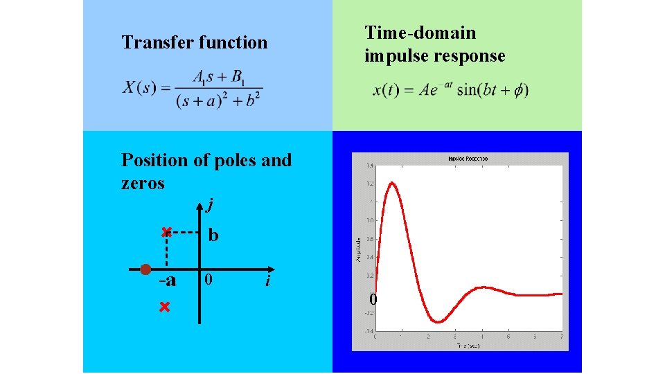
Transfer function Time-domain impulse response Position of poles and zeros j b -a 0 i 0 119

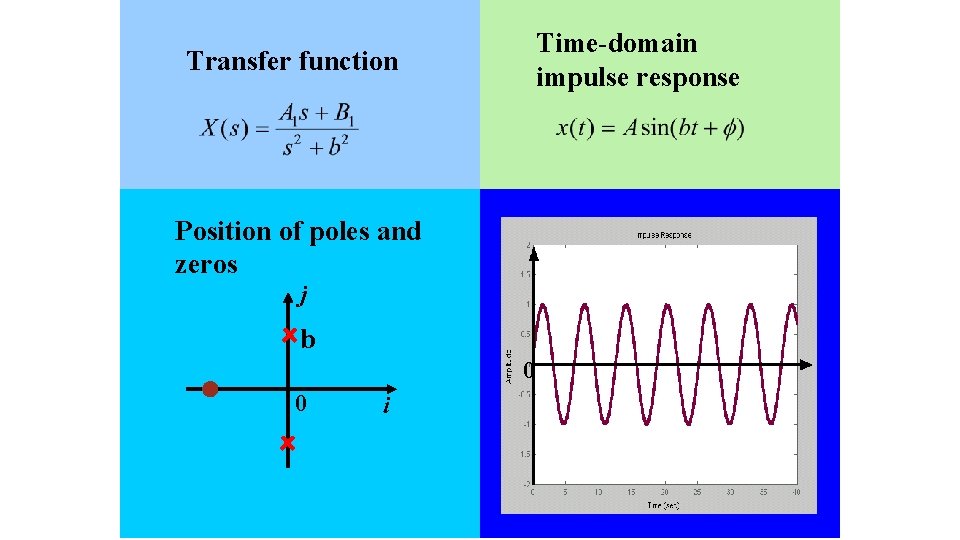
Time-domain impulse response Transfer function Position of poles and zeros j b 0 0 i 120

Time-domain impulse response Transfer function Position of poles and zeros j 0 -a i 121

Transfer function： Time-domain dynamic response Position of poles and zeros j b -a 0 0 i 122

Summary of pole position & system dynamics 123

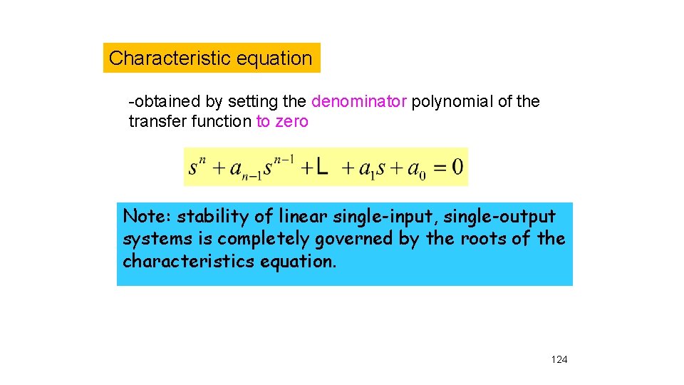
Characteristic equation -obtained by setting the denominator polynomial of the transfer function to zero Note: stability of linear single-input, single-output systems is completely governed by the roots of the characteristics equation. 124

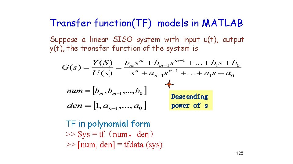
Transfer function(TF) models in MATLAB Suppose a linear SISO system with input u(t), output y(t), the transfer function of the system is Descending power of s TF in polynomial form >> Sys = tf（num，den） >> [num, den] = tfdata (sys) 125

TF in zero-pole form >> sys = zpk（z, p, k） >> [z, p, k] = tfdata (sys) Transform TS from zero-pole form into polynomial form >> [z, p, k] = tf 2 zp(num, den) 126

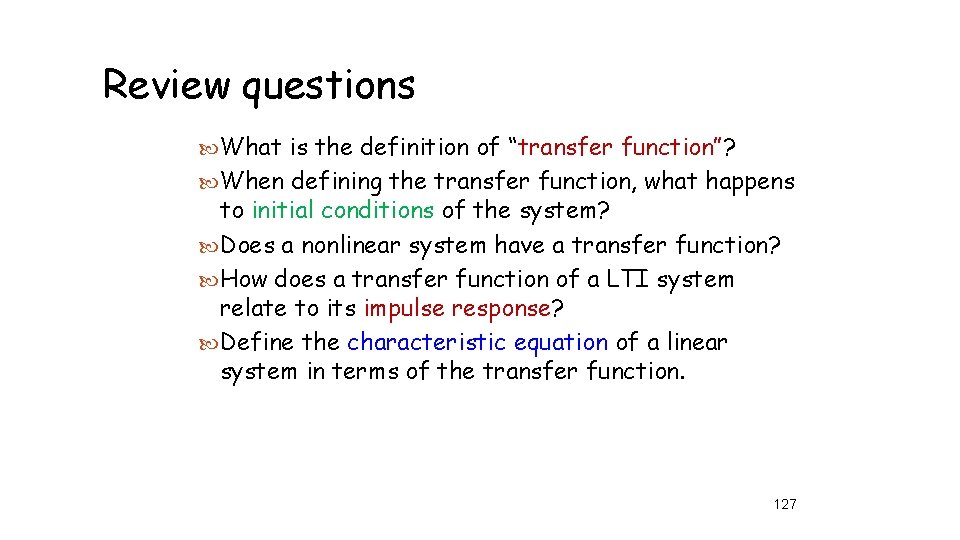
Review questions What is the definition of “transfer function”? When defining the transfer function, what happens to initial conditions of the system? Does a nonlinear system have a transfer function? How does a transfer function of a LTI system relate to its impulse response? Define the characteristic equation of a linear system in terms of the transfer function. 127

Block diagram 128

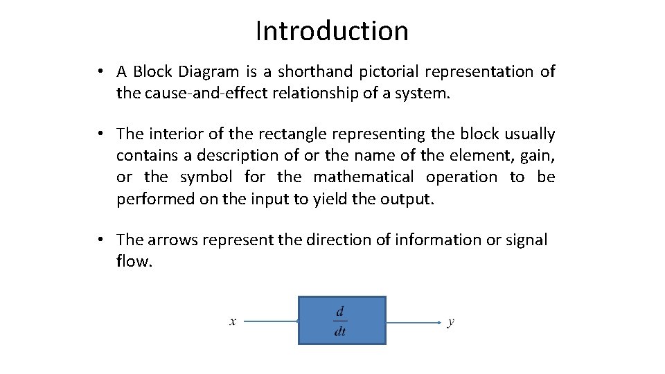
Introduction • A Block Diagram is a shorthand pictorial representation of the cause-and-effect relationship of a system. • The interior of the rectangle representing the block usually contains a description of or the name of the element, gain, or the symbol for the mathematical operation to be performed on the input to yield the output. • The arrows represent the direction of information or signal flow.

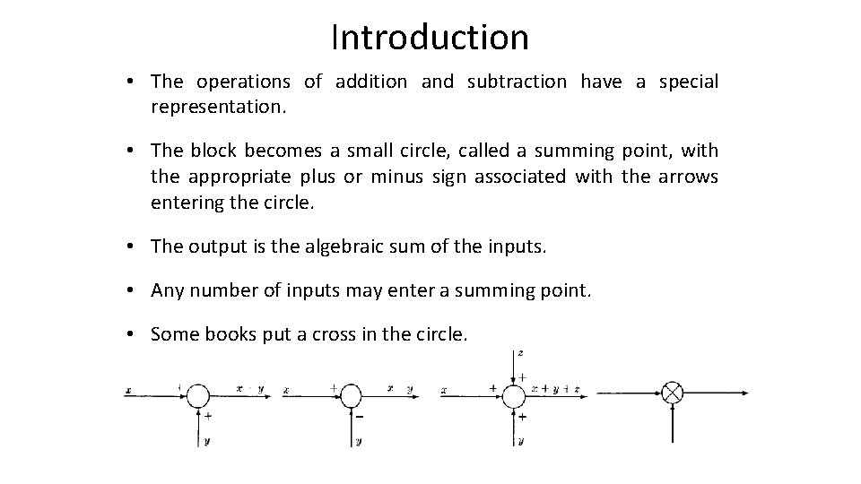
Introduction • The operations of addition and subtraction have a special representation. • The block becomes a small circle, called a summing point, with the appropriate plus or minus sign associated with the arrows entering the circle. • The output is the algebraic sum of the inputs. • Any number of inputs may enter a summing point. • Some books put a cross in the circle.

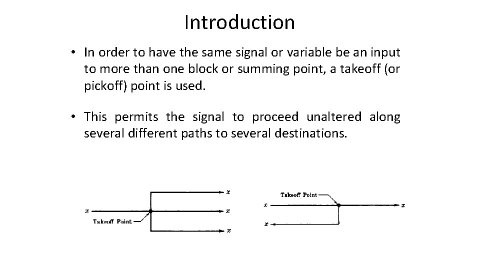
Introduction • In order to have the same signal or variable be an input to more than one block or summing point, a takeoff (or pickoff) point is used. • This permits the signal to proceed unaltered along several different paths to several destinations.

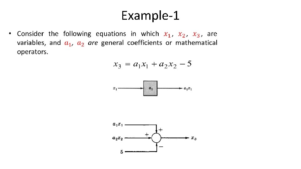
Example-1 •

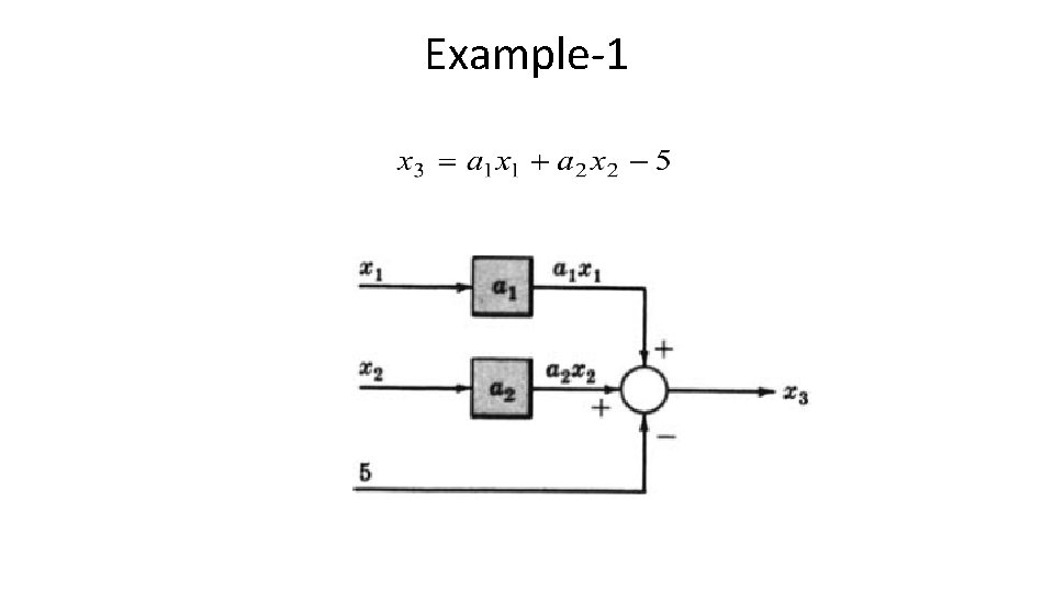
Example-1

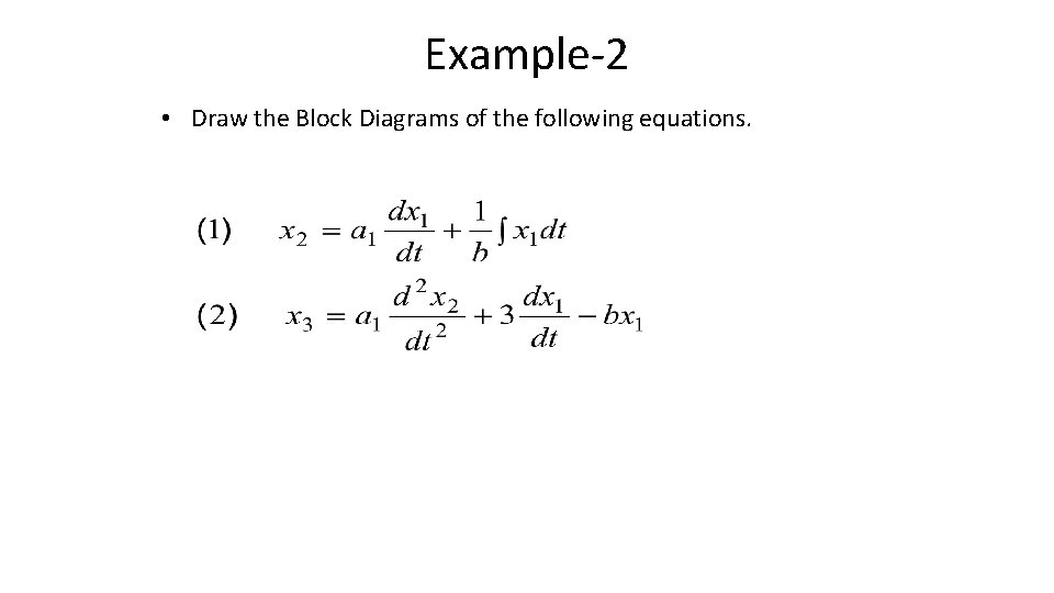
Example-2 • Draw the Block Diagrams of the following equations.

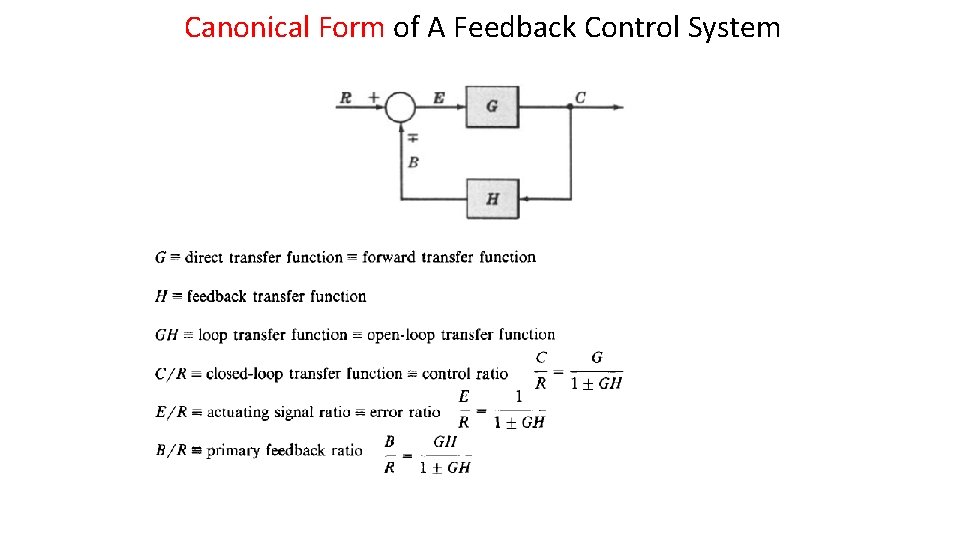
Canonical Form of A Feedback Control System

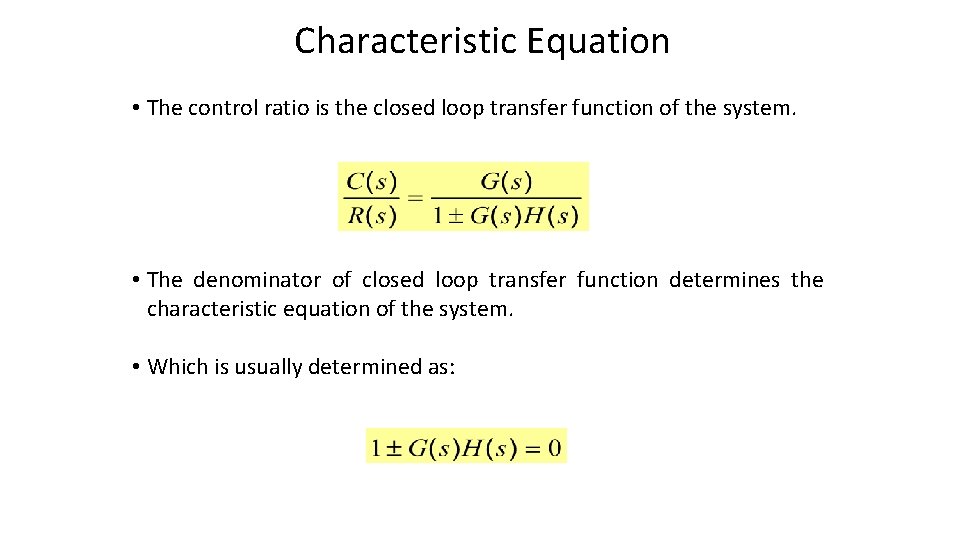
Characteristic Equation • The control ratio is the closed loop transfer function of the system. • The denominator of closed loop transfer function determines the characteristic equation of the system. • Which is usually determined as:

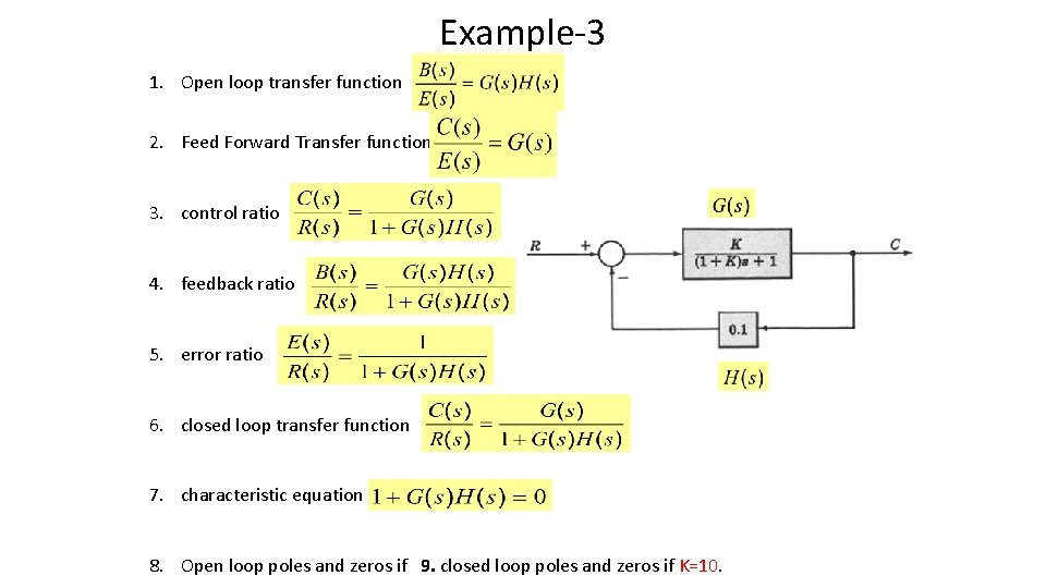
Example-3 1. Open loop transfer function 2. Feed Forward Transfer function 3. control ratio 4. feedback ratio 5. error ratio 6. closed loop transfer function 7. characteristic equation 8. Open loop poles and zeros if 9. closed loop poles and zeros if K=10.

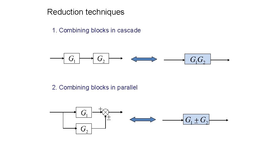
Reduction techniques 1. Combining blocks in cascade 2. Combining blocks in parallel

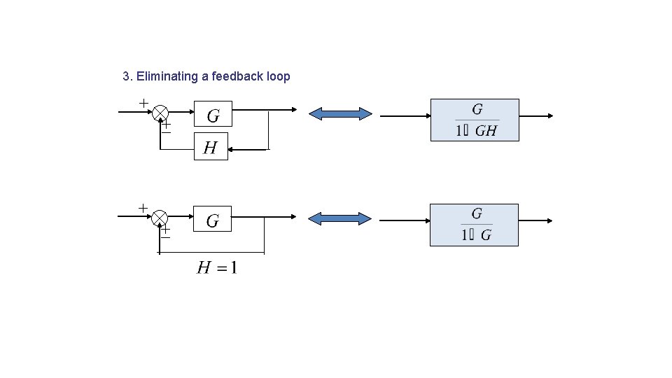
3. Eliminating a feedback loop

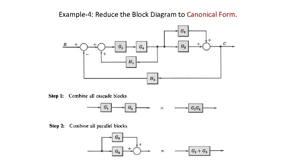
Example-4: Reduce the Block Diagram to Canonical Form.

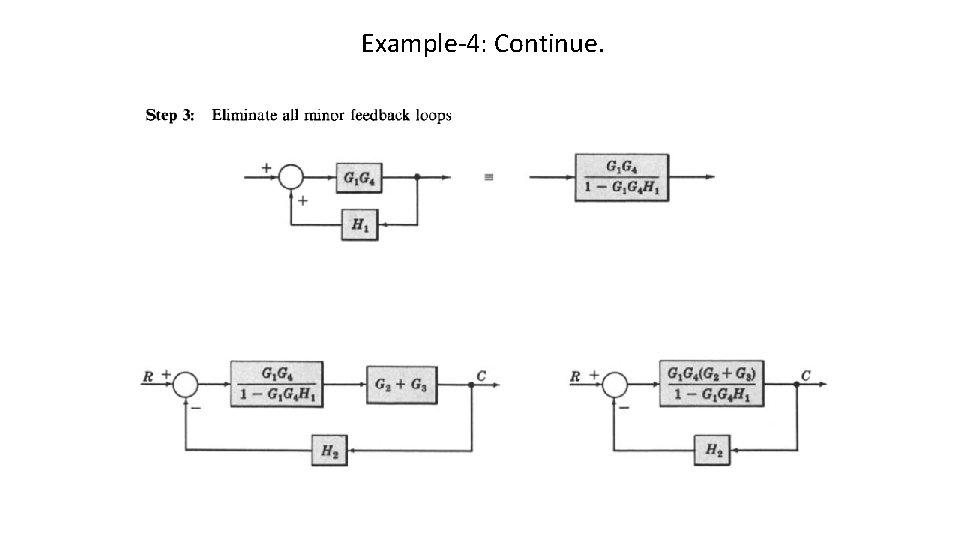
Example-4: Continue.

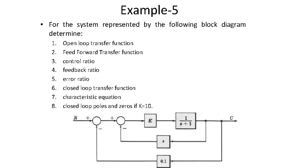
Example-5 • For the system represented by the following block diagram determine: 1. 2. 3. 4. 5. 6. 7. 8. Open loop transfer function Feed Forward Transfer function control ratio feedback ratio error ratio closed loop transfer function characteristic equation closed loop poles and zeros if K=10.

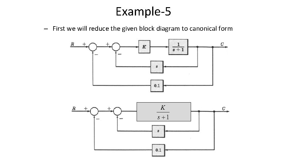
Example-5 – First we will reduce the given block diagram to canonical form

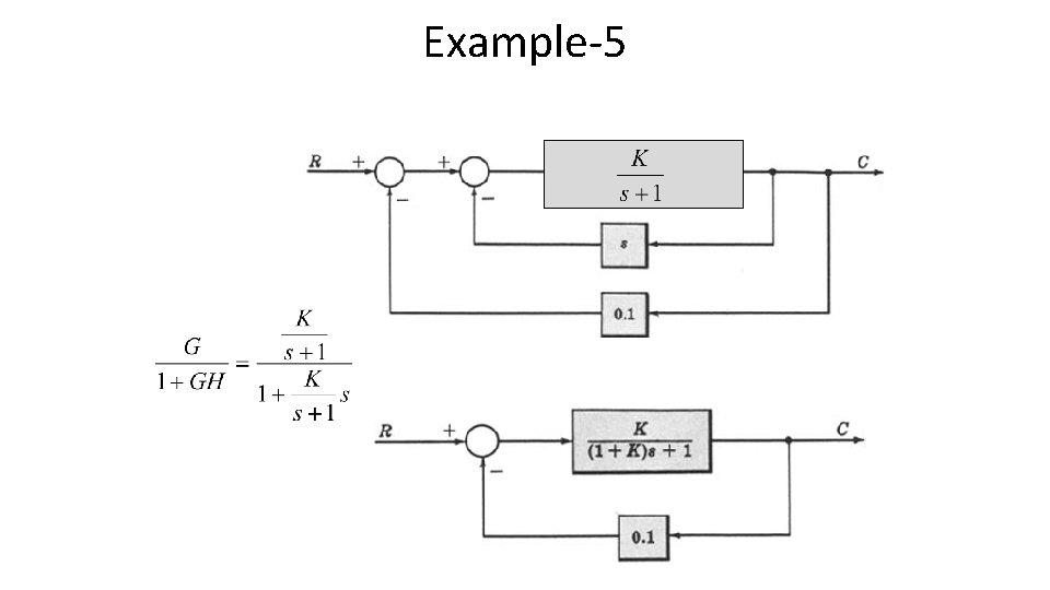
Example-5

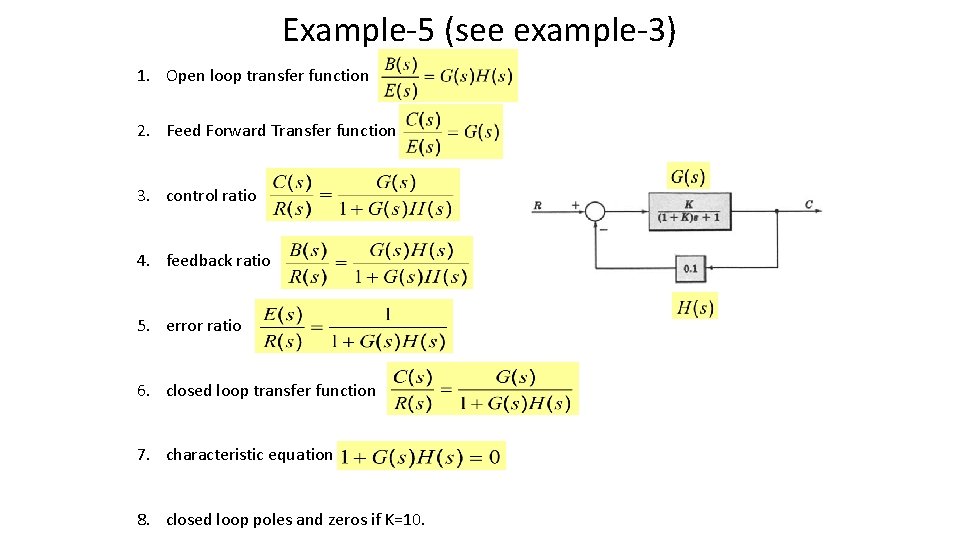
Example-5 (see example-3) 1. Open loop transfer function 2. Feed Forward Transfer function 3. control ratio 4. feedback ratio 5. error ratio 6. closed loop transfer function 7. characteristic equation 8. closed loop poles and zeros if K=10.

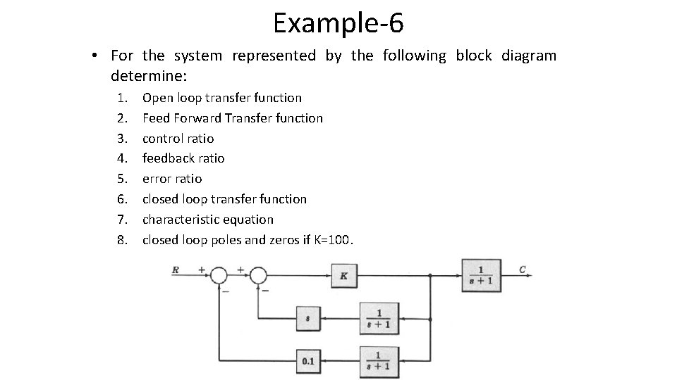
Example-6 • For the system represented by the following block diagram determine: 1. 2. 3. 4. 5. 6. 7. 8. Open loop transfer function Feed Forward Transfer function control ratio feedback ratio error ratio closed loop transfer function characteristic equation closed loop poles and zeros if K=100.

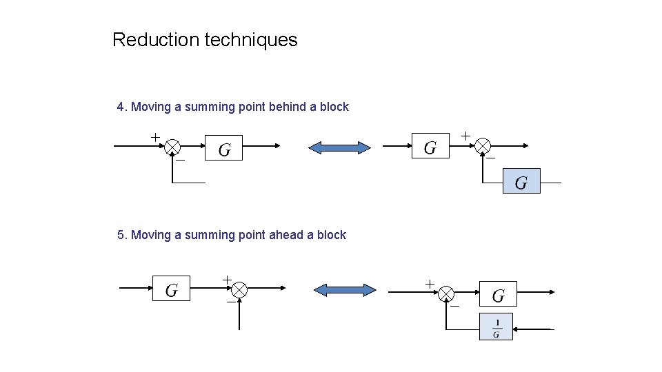
Reduction techniques 4. Moving a summing point behind a block 5. Moving a summing point ahead a block

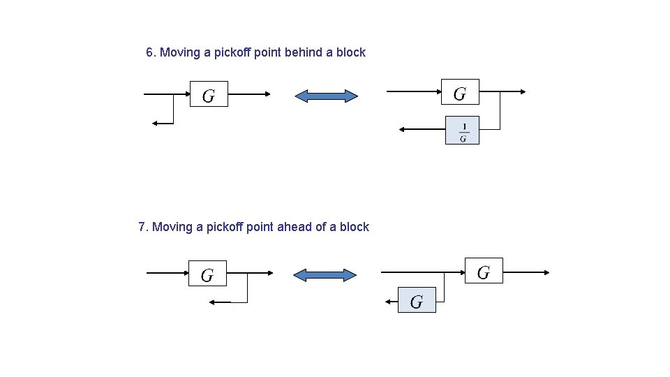
6. Moving a pickoff point behind a block 7. Moving a pickoff point ahead of a block

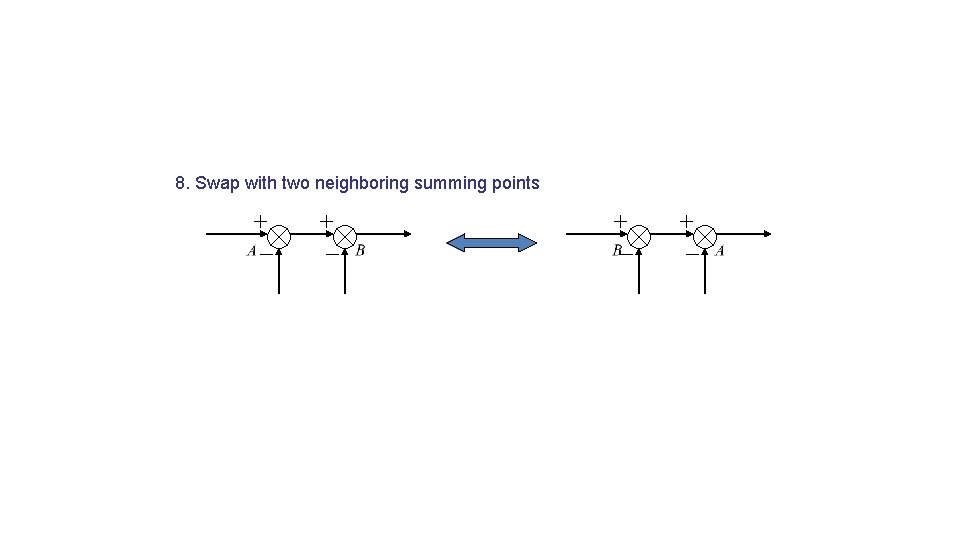
8. Swap with two neighboring summing points

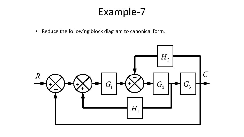
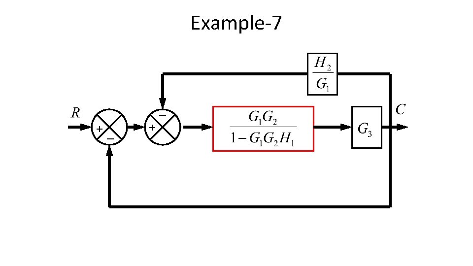
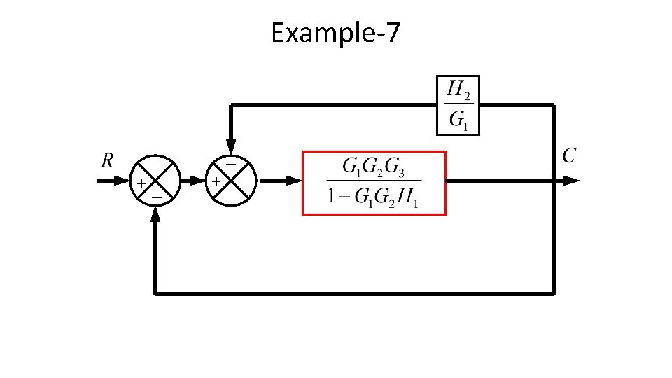
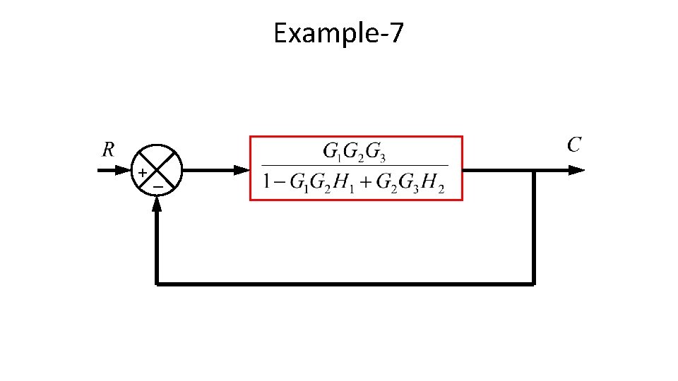
Example-7 • Reduce the following block diagram to canonical form. _ +_ + + +

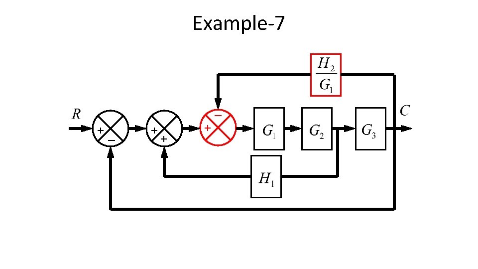
Example-7 _ +_ + + +

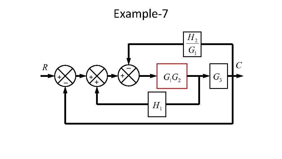
Example-7 _ +_ + + +

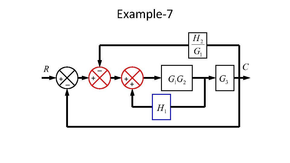
Example-7 _ +_ + + +

Example-7 _ +_ +

Example-7 _ +_ +

Example-7 +_

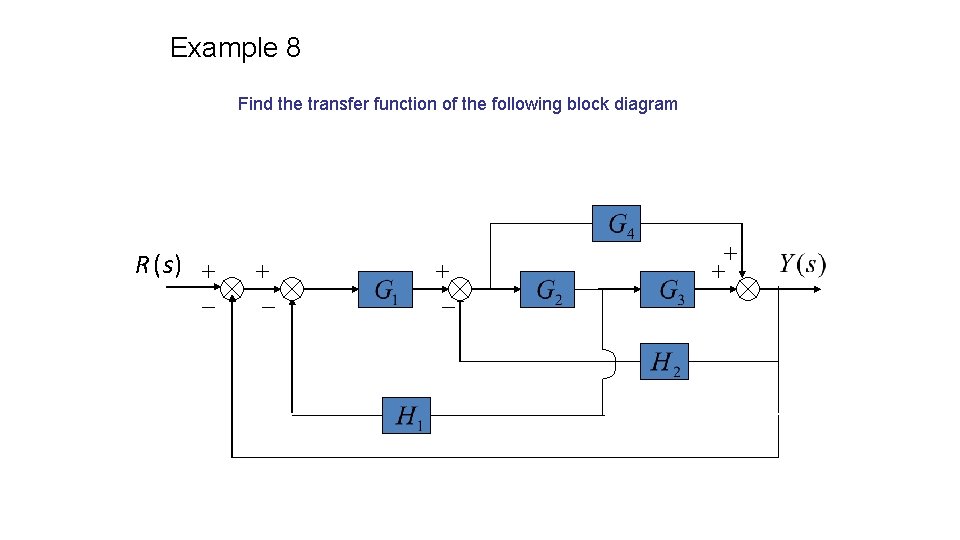
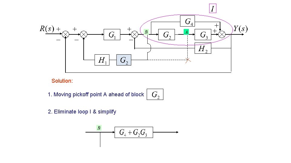
Example 8 Find the transfer function of the following block diagram R (s )

Solution: 1. Moving pickoff point A ahead of block 2. Eliminate loop I & simplify

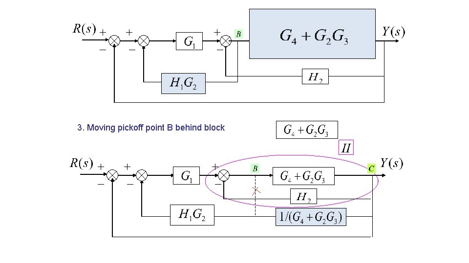
3. Moving pickoff point B behind block

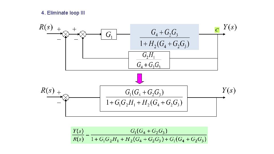
4. Eliminate loop III

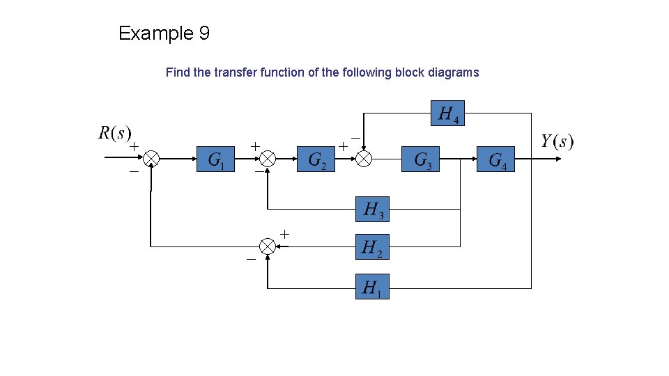
Example 9 Find the transfer function of the following block diagrams

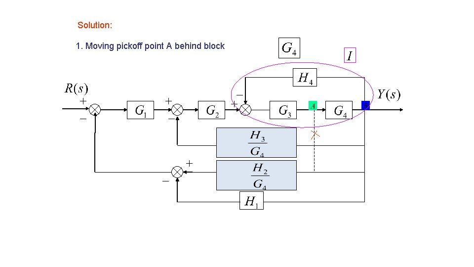
Solution: 1. Moving pickoff point A behind block

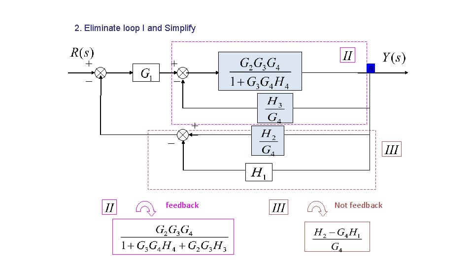
2. Eliminate loop I and Simplify feedback Not feedback

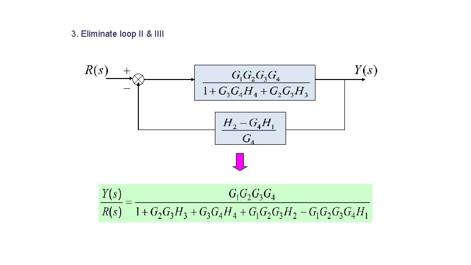
3. Eliminate loop II & IIII

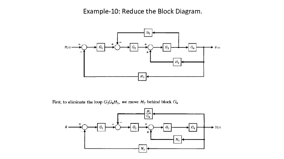
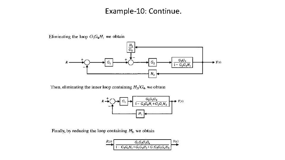
Example-10: Reduce the Block Diagram.

Example-10: Continue.

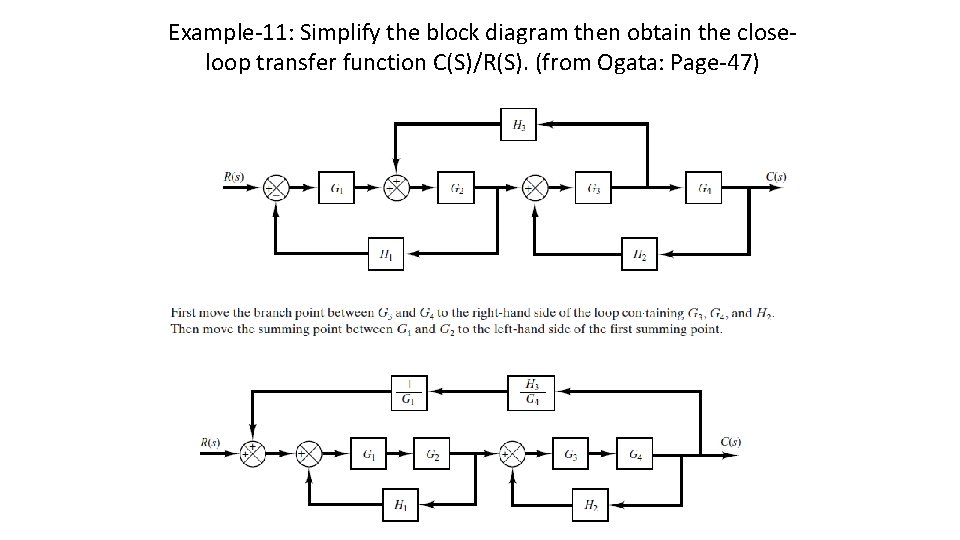
Example-11: Simplify the block diagram then obtain the closeloop transfer function C(S)/R(S). (from Ogata: Page-47)

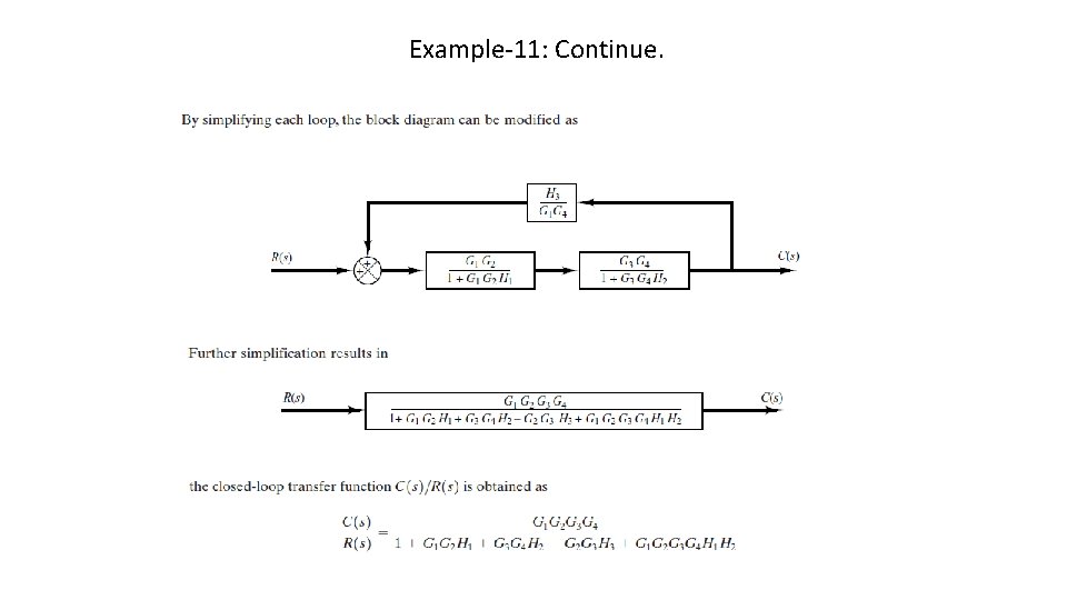
Example-11: Continue.

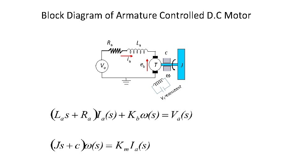
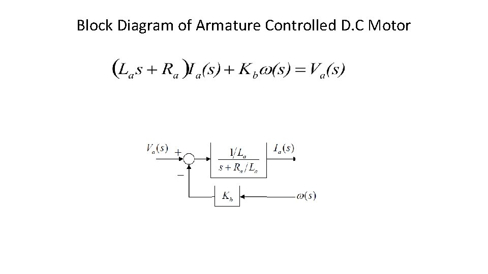
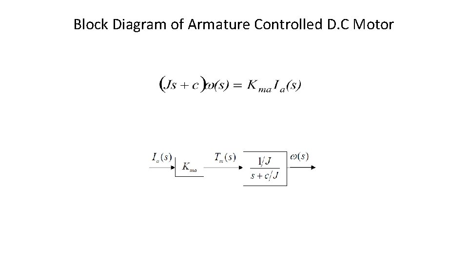
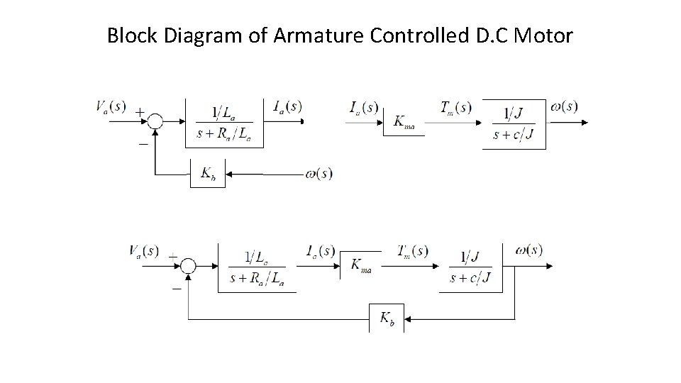
Block Diagram of Armature Controlled D. C Motor Ra Va La ia c eb T J t an t s n =co Vf

Block Diagram of Armature Controlled D. C Motor

Block Diagram of Armature Controlled D. C Motor

Block Diagram of Armature Controlled D. C Motor

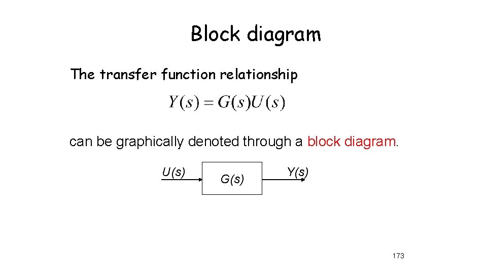
Block diagram The transfer function relationship can be graphically denoted through a block diagram. U(s) G(s) Y(s) 173

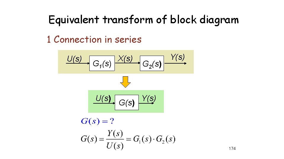
Equivalent transform of block diagram 1 Connection in series U(s) G 1(s) U(s) X(s) G 2(s) Y(s) 174

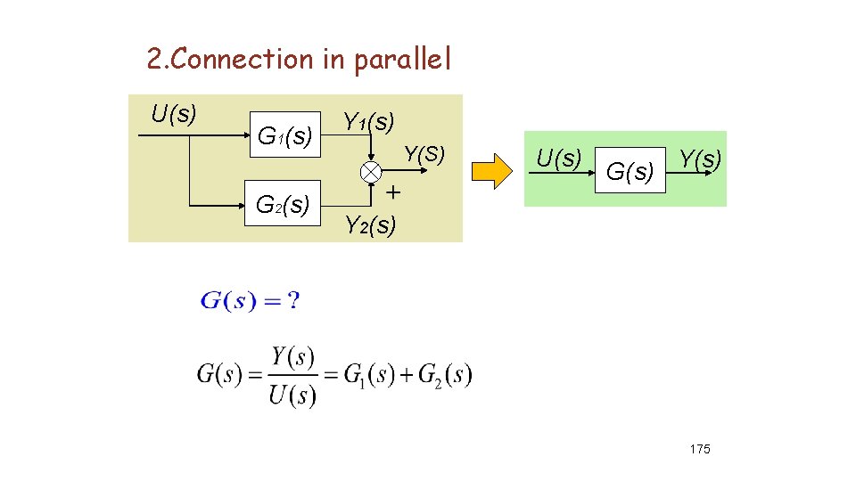
2. Connection in parallel U(s) G 1(s) G 2(s) Y 1(s) Y(S) U(s) G(s) Y 2(s) 175

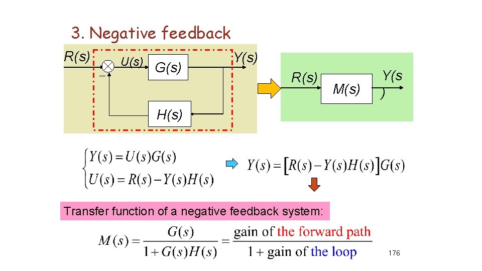
3. Negative feedback R(s) _ U(s) G(s) Y(s) R(s) M(s) Y(s ) H(s) Transfer function of a negative feedback system: 176