Digital Control Systems DCS Lecture11 12 13 Design

Digital Control Systems (DCS) Lecture-11 -12 -13 Design of Control Systems in Sate Space Dr. Imtiaz Hussain Associate Professor Mehran University of Engineering & Technology Jamshoro, Pakistan email: imtiaz. hussain@faculty. muet. edu. pk URL : http: //imtiazhussainkalwar. weebly. com/ 1

Lecture Outline • Introduction • Controllability & Observability • Pole Placement – Topology of Pole Placement – Pole Placement Design Techniques • Using Transformation Matrix P • Direct Substitution Method • Ackermann’s Formula

Introduction • One of the drawbacks of frequency domain methods of design is that after designing the location of the dominant second-order pair of poles, we keep our fingers crossed, hoping that the higher-order poles do not affect the second-order approximation. • What we would like to be able to do is specify all closed-loop poles of the higher-order system.

Introduction • Frequency domain methods of design do not allow us to specify all poles in systems of order higher than 2 because they do not allow for a sufficient number of unknown parameters to place all of the closed-loop poles uniquely. • One gain to adjust, or compensator pole and zero to select, does not yield a sufficient number of parameters to place all the closed-loop poles at desired locations.

Introduction • Remember, to place n unknown quantities, you need n adjustable parameters. • State-space methods solve this problem by introducing into the system – Other adjustable parameters and – The technique for finding these parameter values • On the other hand, state-space methods do not allow the specification of closed-loop zero locations, which frequency domain methods do allow through placement of the lead compensator zero.

Introduction • Finally, there is a wide range of computational support for state-space methods; many software packages support the matrix algebra required by the design process. • However, as mentioned before, the advantages of computer support are balanced by the loss of graphic insight into a design problem that the frequency domain methods yield.

State Controllability • A system is completely controllable if there exists an unconstrained control u(t) that can transfer any initial state x(to) to any other desired location x(t) in a finite time, to ≤ t ≤ T. uncontrollable

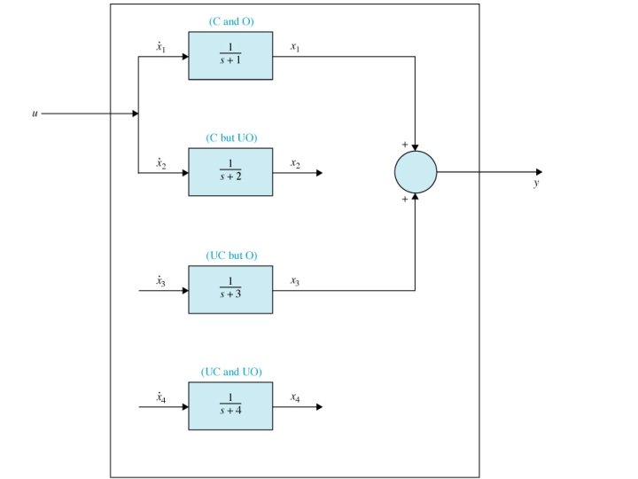
State Controllability (Example) • Consider the system given below • State diagram of the system is

State Controllability (Example) •

State Observability • A system is completely observable if and only if there exists a finite time T such that the initial state x(0) can be determined from the observation history y(t) given the control u(t), 0≤ t ≤ T. observable unobservable

State Observability • Observable Matrix (OM) • The system is said to be completely state observable if

State Observability (Example) • Consider the system given below • OM is obtained as • Where

State Observability (Example) •

Home Work • Check the state controllability, state observability and output controllability of the following system

Pole Placement • In this lecture we will discuss a design method commonly called the pole-placement or pole-assignment technique. • We assume that all state variables are measurable and are available for feedback. • If the system considered is completely state controllable, then poles of the closed-loop system may be placed at any desired locations by means of state feedback through an appropriate state feedback gain matrix.

Pole Placement • The present design technique begins with a determination of the desired closed-loop poles based on the transientresponse and/or frequency-response requirements, such as speed, damping ratio, or bandwidth, as well as steadystate requirements. • By choosing an appropriate gain matrix for state feedback, it is possible to force the system to have closed-loop poles at the desired locations, provided that the original system is completely state controllable.

Topology of Pole Placement • Consider a plant represented in state space by

Topology of Pole Placement • In a typical feedback control system, the output, y, is fed back to the summing junction. • It is now that the topology of the design changes. Instead of feeding back y, we feed back all of the state variables. • If each state variable is fed back to the control, u, through a gain, ki, there would be n gains, ki, that could be adjusted to yield the required closed-loop pole values.

Topology of Pole Placement • The feedback through the gains, ki, is represented in following figure by the feedback vector K.

Topology of Pole Placement • For example consider a plant signal-flow graph in phasevariable form

Topology of Pole Placement • Each state variable is then fed back to the plant’s input, u, through a gain, ki, as shown in Figure

Pole Placement • We will limit our discussions to single-input, single-output systems (i. e. we will assume that the control signal u(t) and output signal y(t) to be scalars). • We will also assume that the reference input r(t) is zero.

Pole Placement • The stability and transient response characteristics are determined by the eigenvalues of matrix A-BK. • If matrix K is chosen properly Eigenvalues of the system can be placed at desired location. • And the problem of placing the regulator poles (closedloop poles) at the desired location is called a poleplacement problem.

Pole Placement • There are three approaches that can be used to determine the gain matrix K to place the poles at desired location. • Using Transformation Matrix P • Direct Substitution Method • Ackermann’s formula • All those method yields the same result.

Pole Placement (Using Transformation Matrix P) • Following are the steps to be followed in this particular method. 1. Check the state controllability of the system

Pole Placement (Using Transformation Matrix P) • Following are the steps to be followed in this particular method. 2. Transform the given system in CCF.

Pole Placement (Using Transformation Matrix P) •

Pole Placement (Using Transformation Matrix P) • Following are the steps to be followed in this particular method. 4. Compute the gain matrix K.

Pole Placement (Using Transformation Matrix P) • Example-1: Consider the regulator system shown in following figure. The plant is given by

Pole Placement (Using Transformation Matrix P) • Example-1: Step-1 • First, we need to check the controllability matrix of the system. Since the controllability matrix CM is given by • We find that rank(CM)=3. Thus, the system is completely state controllable and arbitrary pole placement is possible.

Pole Placement (Using Transformation Matrix P) • Example-1: Step-2 (Transformation to CCF) • The given system is already in CCF

Pole Placement (Using Transformation Matrix P) • Example-1: Step-3 • Determine the characteristic equation • Hence

Pole Placement (Using Transformation Matrix P) •

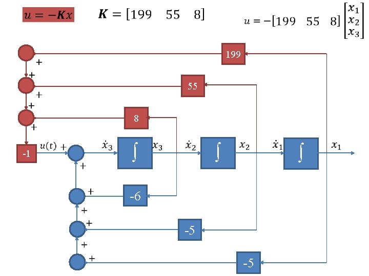
Pole Placement (Using Transformation Matrix P) • Example-1: Step-4 • State feedback gain matric K is then calculated as

Pole Placement (Using Transformation Matrix P) • State diagram of the given system ∫ ∫ -6 -5 -1 ∫

Pole Placement (Direct Substitution Method) • Following are the steps to be followed in this particular method. 1. Check the state controllability of the system

Pole Placement (Direct Substitution Method) •

Pole Placement (Using Direct Substitution) • Example-1: Consider the regulator system shown in following figure. The plant is given by

Pole Placement (Using Transformation Matrix P) • Example-1: Step-1 • First, we need to check the controllability matrix of the system. Since the controllability matrix CM is given by • We find that rank(CM)=3. Thus, the system is completely state controllable and arbitrary pole placement is possible.

Pole Placement (Using Transformation Matrix P) • Example-1: Step-2 • Let K be • Desired characteristic polynomial is obtained as • Comparing the coefficients of powers of s

Pole Placement (Ackermann’s Formula) • Following are the steps to be followed in this particular method. 1. Check the state controllability of the system

Pole Placement (Ackermann’s Formula) • Following are the steps to be followed in this particular method. 2. Use Ackermann’s formula to calculate K

Pole Placement (Ackermann’s Formula) • Example-1: Consider the regulator system shown in following figure. The plant is given by

Pole Placement (Using Transformation Matrix P) • Example-1: Step-1 • First, we need to check the controllability matrix of the system. Since the controllability matrix CM is given by • We find that rank(CM)=3. Thus, the system is completely state controllable and arbitrary pole placement is possible.

Pole Placement (Ackermann’s Formula) • Following are the steps to be followed in this particular method. 2. Use Ackermann’s formula to calculate K

Pole Placement (Ackermann’s Formula)

Pole Placement (Ackermann’s Formula)

Pole Placement • Example-2: Consider the regulator system shown in following figure. The plant is given by • Determine the state feedback gain for each state variable to place the poles at -1+j, -1 -j, -3. (Apply all methods)

To download this lecture visit http: //imtiazhussainkalwar. weebly. com/ END OF LECTURES-12 -13 -14