COE 561 Digital System Design Synthesis MultipleLevel Logic

COE 561 Digital System Design & Synthesis Multiple-Level Logic Synthesis Dr. Aiman H. El-Maleh Computer Engineering Department King Fahd University of Petroleum & Minerals [Adapted from slides of Prof. G. De Micheli: Synthesis & Optimization of Digital Circuits]

Outline … n n Representations. Taxonomy of optimization methods. • Goals: area/delay. • Algorithms: Algebraic/Boolean. • Rule-based methods. Examples of transformations. Algebraic model. • Algebraic division. • Algebraic substitution. • Single-cube extraction. • Multiple-cube extraction. • Decomposition. • Factorization. • Fast extraction. 2

… Outline n External and internal don’t care sets. n Boolean simplification and substitution. n Testability properties of multiple-level logic. n Synthesis for testability. n Network delay modeling. n Algorithms for delay minimization. n Transformations for delay reduction. • Controllability don’t care sets. • Observability don’t care sets. 3

Motivation n Combinational logic circuits very often implemented as multiple-level networks of logic gates. Provides several degrees of freedom in logic design • Exploited in optimizing area and delay. • Different timing requirements on input/output paths. Multiple-level networks viewed as interconnection of single-output gates • Single type of gate (e. g. NANDs or NORs). • Instances of a cell library. • Macro cells. n Multilevel optimization is divided into two tasks • Optimization neglecting implementation constraints assuming loose models of area and delay. • Constraints on the usable gates are taken into account during optimization. 4

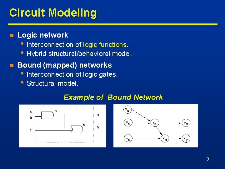
Circuit Modeling n Logic network n Bound (mapped) networks • Interconnection of logic functions. • Hybrid structural/behavioral model. • Interconnection of logic gates. • Structural model. Example of Bound Network 5

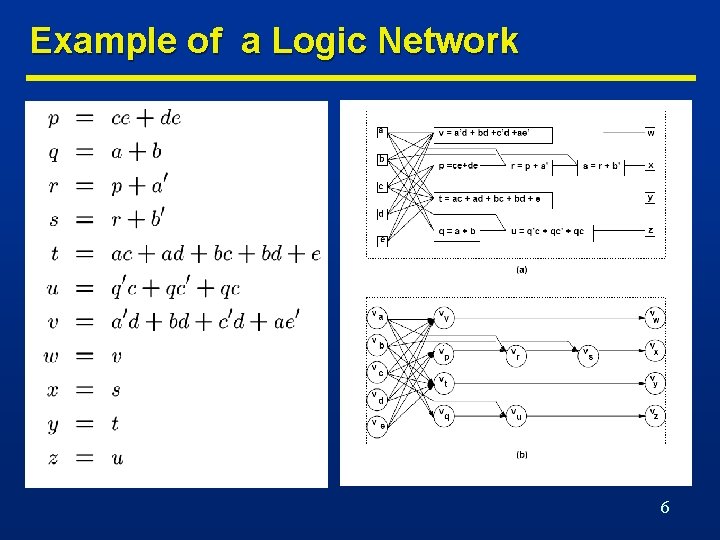
Example of a Logic Network 6

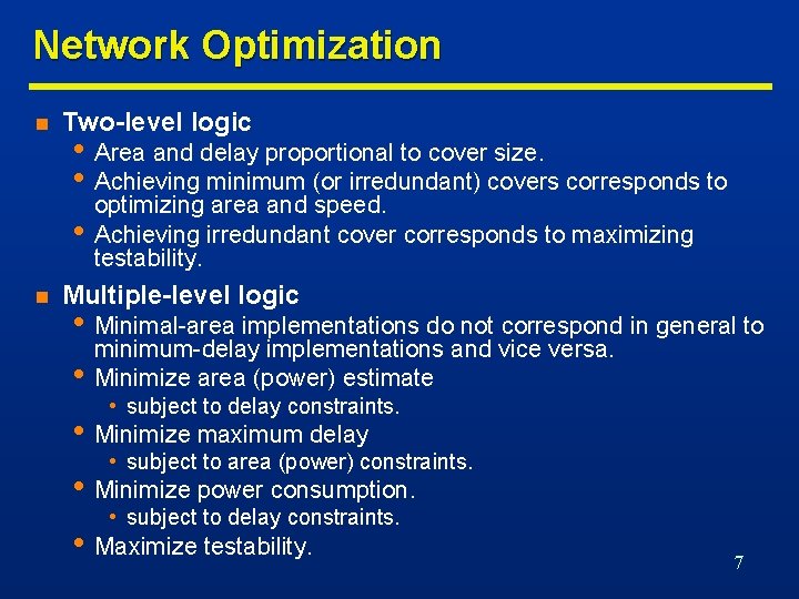
Network Optimization n Two-level logic • Area and delay proportional to cover size. • Achieving minimum (or irredundant) covers corresponds to optimizing area and speed. • Achieving irredundant cover corresponds to maximizing testability. n Multiple-level logic • Minimal-area implementations do not correspond in general to minimum-delay implementations and vice versa. • Minimize area (power) estimate • subject to delay constraints. • Minimize maximum delay • subject to area (power) constraints. • Minimize power consumption. • subject to delay constraints. • Maximize testability. 7

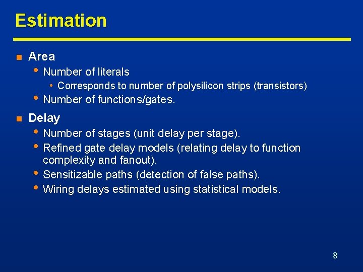
Estimation n Area • Number of literals • Corresponds to number of polysilicon strips (transistors) • Number of functions/gates. n Delay • Number of stages (unit delay per stage). • Refined gate delay models (relating delay to function • • complexity and fanout). Sensitizable paths (detection of false paths). Wiring delays estimated using statistical models. 8

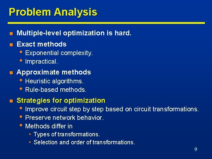
Problem Analysis n Multiple-level optimization is hard. n Exact methods n Approximate methods n Strategies for optimization • Exponential complexity. • Impractical. • Heuristic algorithms. • Rule-based methods. • Improve circuit step by step based on circuit transformations. • Preserve network behavior. • Methods differ in • Types of transformations. • Selection and order of transformations. 9

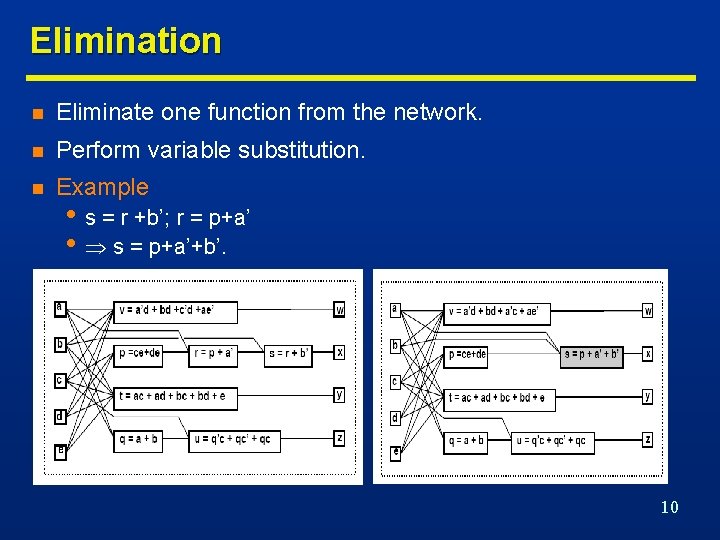
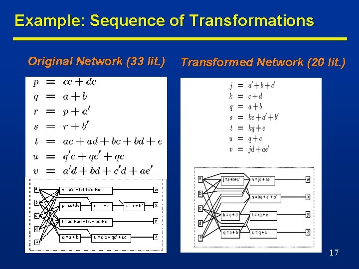
Elimination n Eliminate one function from the network. n Perform variable substitution. n Example • s = r +b’; r = p+a’ • s = p+a’+b’. 10

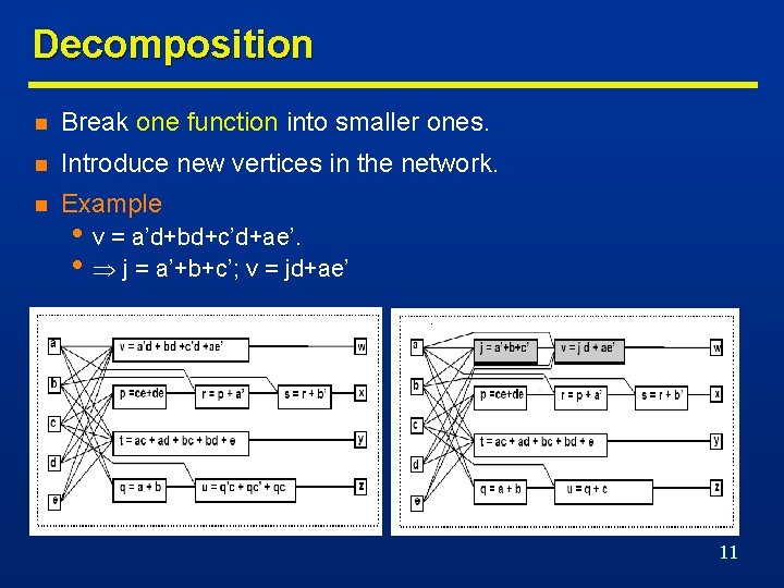
Decomposition n Break one function into smaller ones. n Introduce new vertices in the network. n Example • v = a’d+bd+c’d+ae’. • j = a’+b+c’; v = jd+ae’ 11

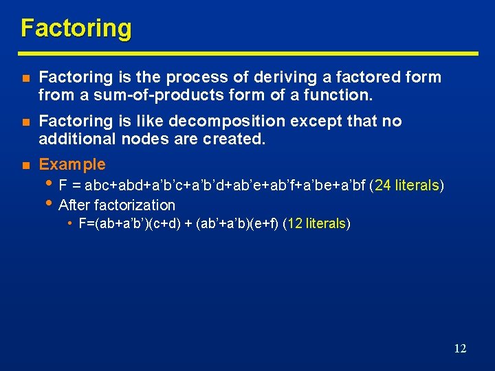
Factoring n Factoring is the process of deriving a factored form from a sum-of-products form of a function. n Factoring is like decomposition except that no additional nodes are created. n Example • F = abc+abd+a’b’c+a’b’d+ab’e+ab’f+a’be+a’bf (24 literals) • After factorization • F=(ab+a’b’)(c+d) + (ab’+a’b)(e+f) (12 literals) 12

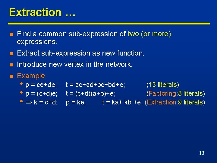
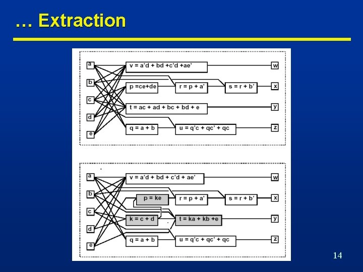
Extraction … n Find a common sub-expression of two (or more) expressions. n Extract sub-expression as new function. n Introduce new vertex in the network. n Example • p = ce+de; • p = (c+d)e; • k = c+d; t = ac+ad+bc+bd+e; (13 literals) t = (c+d)(a+b)+e; (Factoring: 8 literals) p = ke; t = ka+ kb +e; (Extraction: 9 literals) 13

… Extraction 14

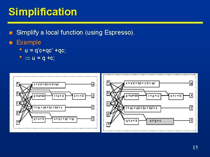
Simplification n Simplify a local function (using Espresso). n Example • • u = q’c+qc’ +qc; u = q +c; 15

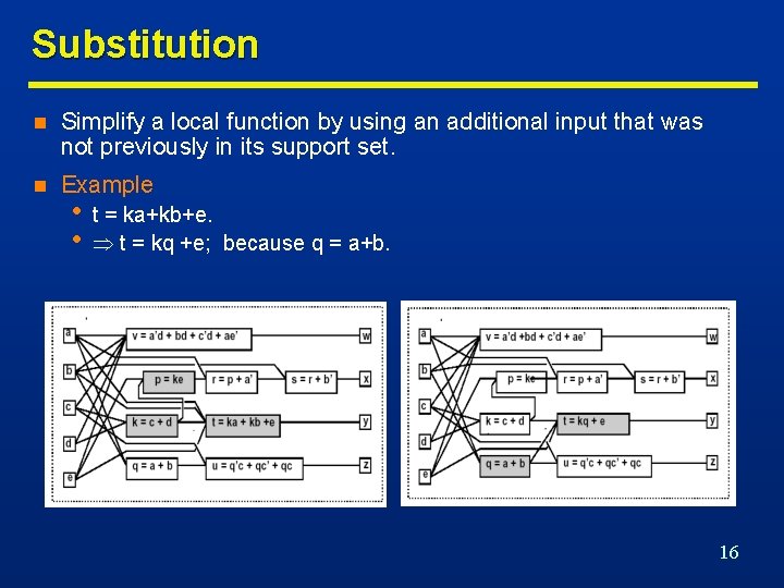
Substitution n Simplify a local function by using an additional input that was not previously in its support set. n Example • • t = ka+kb+e. t = kq +e; because q = a+b. 16

Example: Sequence of Transformations Original Network (33 lit. ) Transformed Network (20 lit. ) 17

Optimization Approaches n Algorithmic approach • Define an algorithm for each transformation type. • Algorithm is an operator on the network. • Each operator has well-defined properties • Heuristic methods still used. • Weak optimality properties. • Sequence of operators • Defined by scripts. • Based on experience. n Rule-based approach (IBM Logic Synthesis System) • Rule-data base • Set of pattern pairs. • Pattern replacement driven by rules. 18

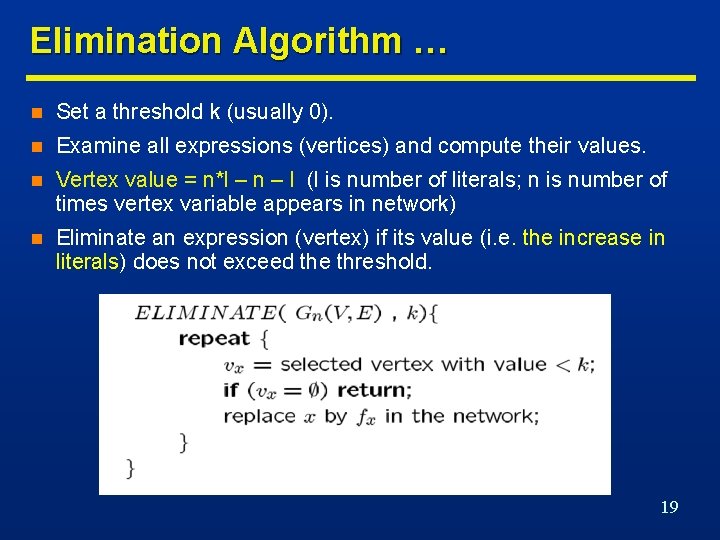
Elimination Algorithm … n Set a threshold k (usually 0). n Examine all expressions (vertices) and compute their values. n Vertex value = n*l – n – l (l is number of literals; n is number of times vertex variable appears in network) n Eliminate an expression (vertex) if its value (i. e. the increase in literals) does not exceed the threshold. 19

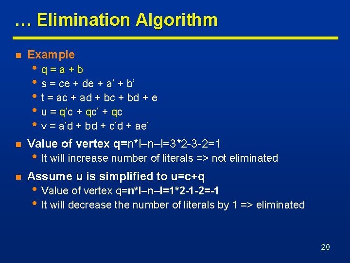
… Elimination Algorithm n Example n Value of vertex q=n*l–n–l=3*2 -3 -2=1 n Assume u is simplified to u=c+q • q=a+b • s = ce + de + a’ + b’ • t = ac + ad + bc + bd + e • u = q’c + qc’ + qc • v = a’d + bd + c’d + ae’ • It will increase number of literals => not eliminated • Value of vertex q=n*l–n–l=1*2 -1 -2=-1 • It will decrease the number of literals by 1 => eliminated 20

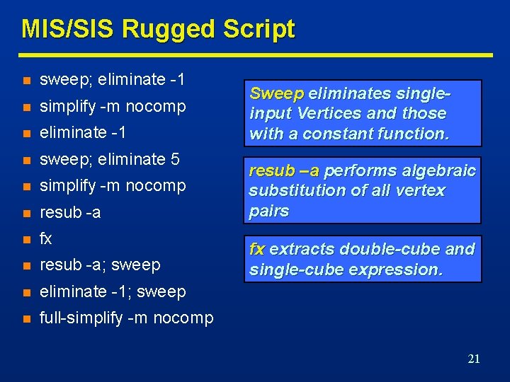
MIS/SIS Rugged Script n sweep; eliminate -1 n simplify -m nocomp n eliminate -1 n sweep; eliminate 5 n simplify -m nocomp n resub -a n fx n resub -a; sweep n eliminate -1; sweep n full-simplify -m nocomp Sweep eliminates singleinput Vertices and those with a constant function. resub –a performs algebraic substitution of all vertex pairs fx extracts double-cube and single-cube expression. 21

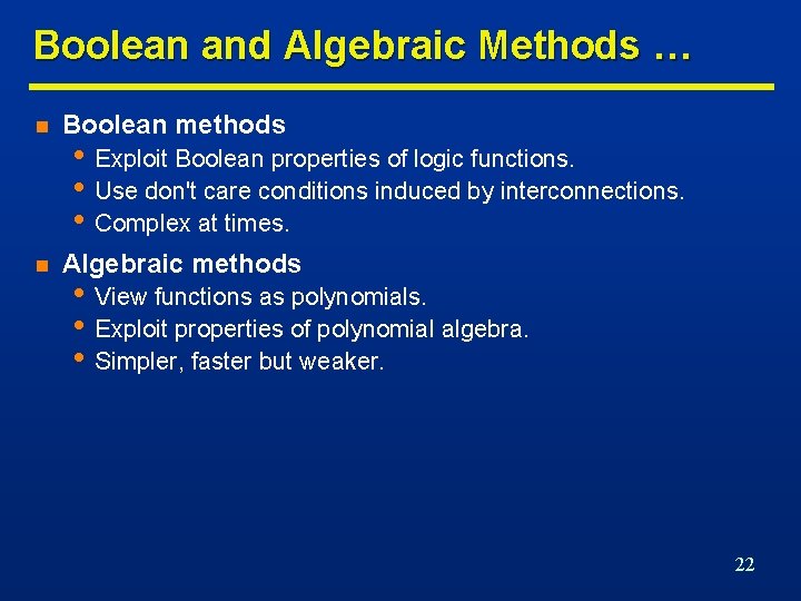
Boolean and Algebraic Methods … n Boolean methods n Algebraic methods • Exploit Boolean properties of logic functions. • Use don't care conditions induced by interconnections. • Complex at times. • View functions as polynomials. • Exploit properties of polynomial algebra. • Simpler, faster but weaker. 22

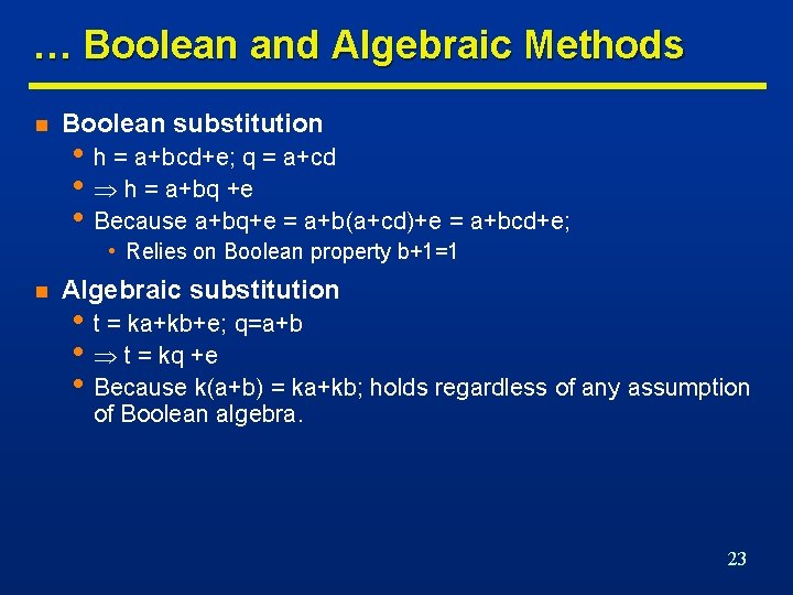
… Boolean and Algebraic Methods n Boolean substitution • h = a+bcd+e; q = a+cd • h = a+bq +e • Because a+bq+e = a+b(a+cd)+e = a+bcd+e; • Relies on Boolean property b+1=1 n Algebraic substitution • t = ka+kb+e; q=a+b • t = kq +e • Because k(a+b) = ka+kb; holds regardless of any assumption of Boolean algebra. 23

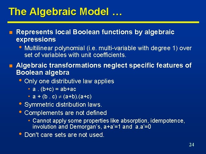
The Algebraic Model … n Represents local Boolean functions by algebraic expressions • Multilinear polynomial (i. e. multi-variable with degree 1) over set of variables with unit coefficients. n Algebraic transformations neglect specific features of Boolean algebra • Only one distributive law applies • a. (b+c) = ab+ac • a + (b. c) (a+b). (a+c) • Symmetric distribution laws. • Complements are not defined • Cannot apply some properties like absorption, idempotence, involution and Demorgan’s, a+a’=1 and a. a’=0 • Don't care sets are not used. 24

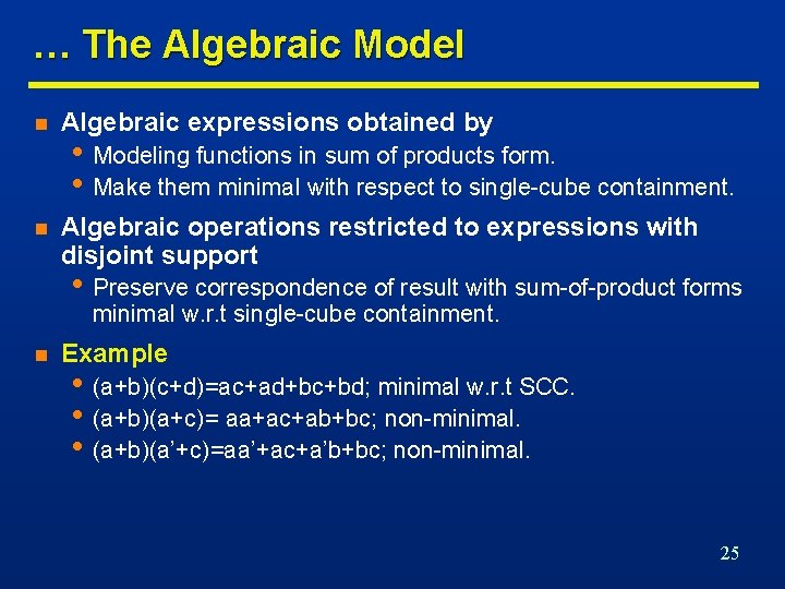
… The Algebraic Model n Algebraic expressions obtained by n Algebraic operations restricted to expressions with disjoint support • Modeling functions in sum of products form. • Make them minimal with respect to single-cube containment. • Preserve correspondence of result with sum-of-product forms minimal w. r. t single-cube containment. n Example • (a+b)(c+d)=ac+ad+bc+bd; minimal w. r. t SCC. • (a+b)(a+c)= aa+ac+ab+bc; non-minimal. • (a+b)(a’+c)=aa’+ac+a’b+bc; non-minimal. 25

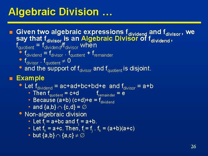
Algebraic Division … n Given two algebraic expressions fdividend and fdivisor , we say that fdivisor is an Algebraic Divisor of fdividend , fquotient = fdividend/fdivisor when • fdividend = fdivisor. fquotient + fremainder • fdivisor. fquotient 0 • and the support of fdivisor and fquotient is disjoint. n Example • Let fdividend = ac+ad+bc+bd+e and fdivisor = a+b • Then fquotient = c+d fremainder = e • Because (a+b) (c+d)+e = fdividend • and {a, b} {c, d} = • Non-algebraic division • Let fi = a+bc and fj = a+b. • Let fk = a+c. Then, fi = fj. fk = (a+b)(a+c) • but {a, b} {a, c} 26

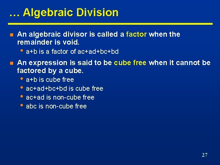
… Algebraic Division n An algebraic divisor is called a factor when the remainder is void. • a+b is a factor of ac+ad+bc+bd n An expression is said to be cube free when it cannot be factored by a cube. • a+b is cube free • ac+ad+bc+bd is cube free • ac+ad is non-cube free • abc is non-cube free 27

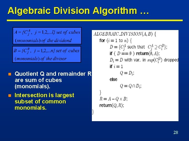
Algebraic Division Algorithm … n Quotient Q and remainder R are sum of cubes (monomials). n Intersection is largest subset of common monomials. 28

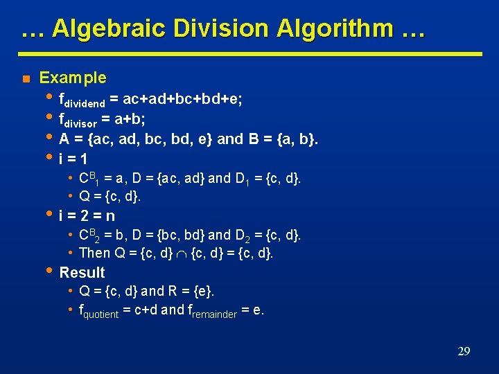
… Algebraic Division Algorithm … n Example • fdividend = ac+ad+bc+bd+e; • fdivisor = a+b; • A = {ac, ad, bc, bd, e} and B = {a, b}. • i=1 • CB 1 = a, D = {ac, ad} and D 1 = {c, d}. • Q = {c, d}. • i=2=n • CB 2 = b, D = {bc, bd} and D 2 = {c, d}. • Then Q = {c, d}. • Result • Q = {c, d} and R = {e}. • fquotient = c+d and fremainder = e. 29

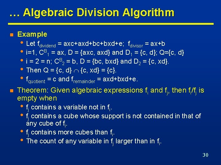
… Algebraic Division Algorithm n Example n Theorem: Given algebraic expressions fi and fj, then fi/fj is empty when • Let fdividend = axc+axd+bc+bxd+e; fdivisor = ax+b • i=1, CB 1 = ax, D = {axc, axd} and D 1 = {c, d}; Q={c, d} • i = 2 = n; CB 2 = b, D = {bc, bxd} and D 2 = {c, xd}. • Then Q = {c, d} {c, xd} = {c}. • fquotient = c and fremainder = axd+bxd+e. • fj contains a variable not in fi. • fj contains a cube whose support is not contained in that of • • any cube of fi. fj contains more cubes than fi. The count of any variable in fj larger than in fi. 30

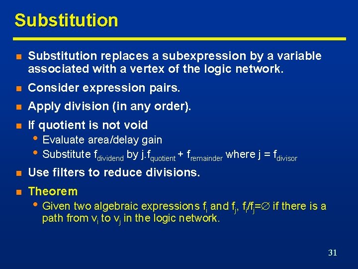
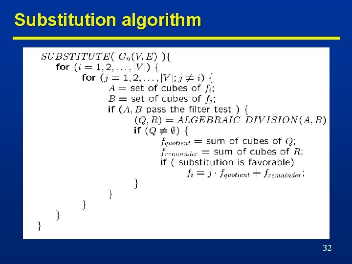
Substitution n Substitution replaces a subexpression by a variable associated with a vertex of the logic network. n Consider expression pairs. n Apply division (in any order). n If quotient is not void n Use filters to reduce divisions. n Theorem • Evaluate area/delay gain • Substitute fdividend by j. fquotient + fremainder where j = fdivisor • Given two algebraic expressions fi and fj, fi/fj= if there is a path from vi to vj in the logic network. 31

Substitution algorithm 32

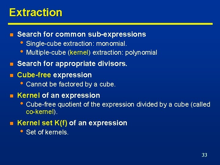
Extraction n Search for common sub-expressions n Search for appropriate divisors. n Cube-free expression n Kernel of an expression • Single-cube extraction: monomial. • Multiple-cube (kernel) extraction: polynomial • Cannot be factored by a cube. • Cube-free quotient of the expression divided by a cube (called co-kernel). n Kernel set K(f) of an expression • Set of kernels. 33

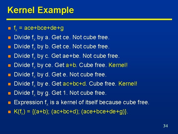
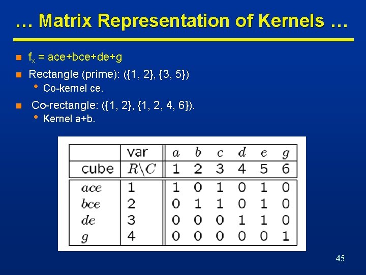
Kernel Example n fx = ace+bce+de+g n Divide fx by a. Get ce. Not cube free. n Divide fx by b. Get ce. Not cube free. n Divide fx by c. Get ae+be. Not cube free. n Divide fx by ce. Get a+b. Cube free. Kernel! n Divide fx by d. Get e. Not cube free. n Divide fx by e. Get ac+bc+d. Cube free. Kernel! n Divide fx by g. Get 1. Not cube free. n Expression fx is a kernel of itself because cube free. n K(fx) = {(a+b); (ac+bc+d); (ace+bce+de+g)}. 34

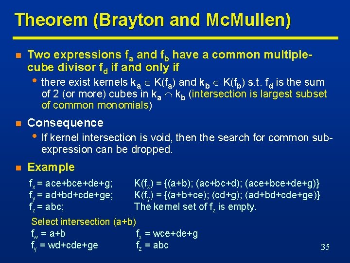
Theorem (Brayton and Mc. Mullen) n Two expressions fa and fb have a common multiplecube divisor fd if and only if • there exist kernels ka K(fa) and kb K(fb) s. t. fd is the sum of 2 (or more) cubes in ka kb (intersection is largest subset of common monomials) n Consequence • If kernel intersection is void, then the search for common subexpression can be dropped. n Example fx = ace+bce+de+g; fy = ad+bd+cde+ge; fz = abc; K(fx) = {(a+b); (ac+bc+d); (ace+bce+de+g)} K(fy) = {(a+b+ce); (cd+g); (ad+bd+cde+ge)} The kernel set of fz is empty. Select intersection (a+b) fw = a+b fx = wce+de+g fy = wd+cde+ge fz = abc 35

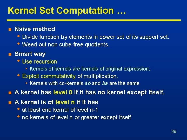
Kernel Set Computation … n Naive method n Smart way • Divide function by elements in power set of its support set. • Weed out non cube-free quotients. • Use recursion • Kernels of kernels are kernels of original expression. • Exploit commutativity of multiplication. • Kernels with co-kernels ab and ba are the same n A kernel has level 0 if it has no kernel except itself. n A kernel is of level n if it has • at least one kernel of level n-1 • no kernels of level n or greater except itself 36

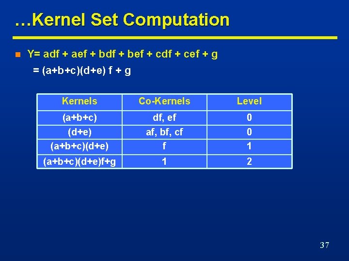
…Kernel Set Computation n Y= adf + aef + bdf + bef + cdf + cef + g = (a+b+c)(d+e) f + g Kernels Co-Kernels Level (a+b+c) df, ef 0 (d+e) (a+b+c)(d+e) af, bf, cf f 0 1 (a+b+c)(d+e)f+g 1 2 37

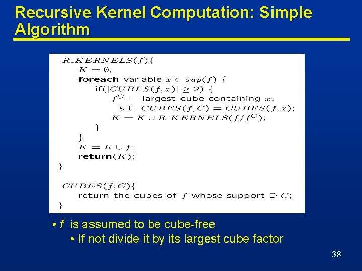
Recursive Kernel Computation: Simple Algorithm • f is assumed to be cube-free • If not divide it by its largest cube factor 38

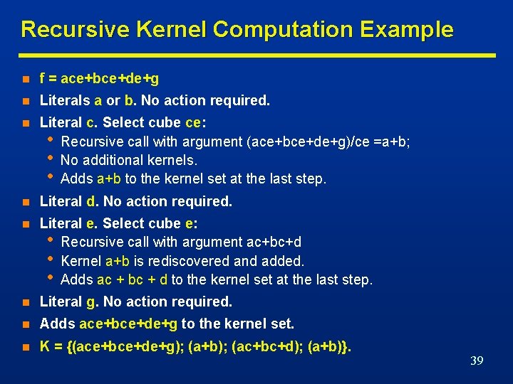
Recursive Kernel Computation Example n f = ace+bce+de+g n Literals a or b. No action required. n Literal c. Select cube ce: • Recursive call with argument (ace+bce+de+g)/ce =a+b; • No additional kernels. • Adds a+b to the kernel set at the last step. n Literal d. No action required. n Literal e. Select cube e: • Recursive call with argument ac+bc+d • Kernel a+b is rediscovered and added. • Adds ac + bc + d to the kernel set at the last step. n Literal g. No action required. n Adds ace+bce+de+g to the kernel set. n K = {(ace+bce+de+g); (a+b); (ac+bc+d); (a+b)}. 39

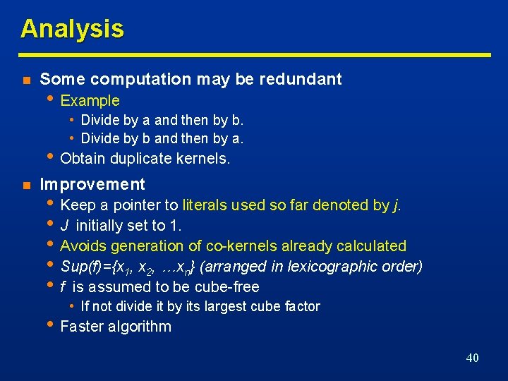
Analysis n Some computation may be redundant • Example • Divide by a and then by b. • Divide by b and then by a. • Obtain duplicate kernels. n Improvement • Keep a pointer to literals used so far denoted by j. • J initially set to 1. • Avoids generation of co-kernels already calculated • Sup(f)={x 1, x 2, …xn} (arranged in lexicographic order) • f is assumed to be cube-free • If not divide it by its largest cube factor • Faster algorithm 40

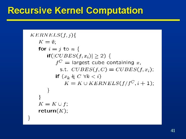
Recursive Kernel Computation 41

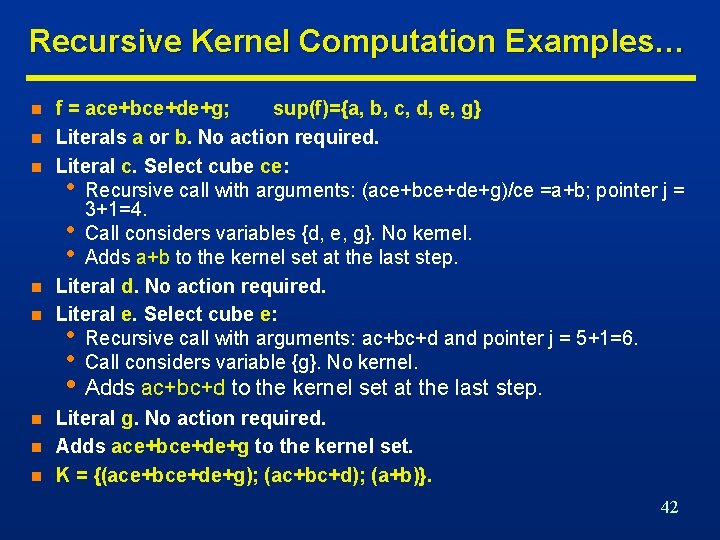
Recursive Kernel Computation Examples… n n n f = ace+bce+de+g; sup(f)={a, b, c, d, e, g} Literals a or b. No action required. Literal c. Select cube ce: • Recursive call with arguments: (ace+bce+de+g)/ce =a+b; pointer j = 3+1=4. • Call considers variables {d, e, g}. No kernel. • Adds a+b to the kernel set at the last step. Literal d. No action required. Literal e. Select cube e: • Recursive call with arguments: ac+bc+d and pointer j = 5+1=6. • Call considers variable {g}. No kernel. • Adds ac+bc+d to the kernel set at the last step. n n n Literal g. No action required. Adds ace+bce+de+g to the kernel set. K = {(ace+bce+de+g); (ac+bc+d); (a+b)}. 42

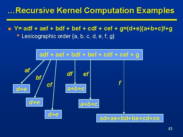
…Recursive Kernel Computation Examples n Y= adf + aef + bdf + bef + cdf + cef + g=(d+e)(a+b+c)f+g • Lexicographic order {a, b, c, d, e, f, g} adf + aef + bdf + bef + cdf + cef + g af df bf cf d+e ef a+b+c d+e ad+ae+bd+be+cd+ce 43

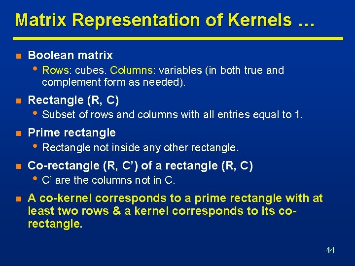
Matrix Representation of Kernels … n Boolean matrix • Rows: cubes. Columns: variables (in both true and complement form as needed). n Rectangle (R, C) n Prime rectangle n Co-rectangle (R, C’) of a rectangle (R, C) n A co-kernel corresponds to a prime rectangle with at least two rows & a kernel corresponds to its corectangle. • Subset of rows and columns with all entries equal to 1. • Rectangle not inside any other rectangle. • C’ are the columns not in C. 44

… Matrix Representation of Kernels … n fx = ace+bce+de+g n Rectangle (prime): ({1, 2}, {3, 5}) n • Co-kernel ce. Co-rectangle: ({1, 2}, {1, 2, 4, 6}). • Kernel a+b. 45

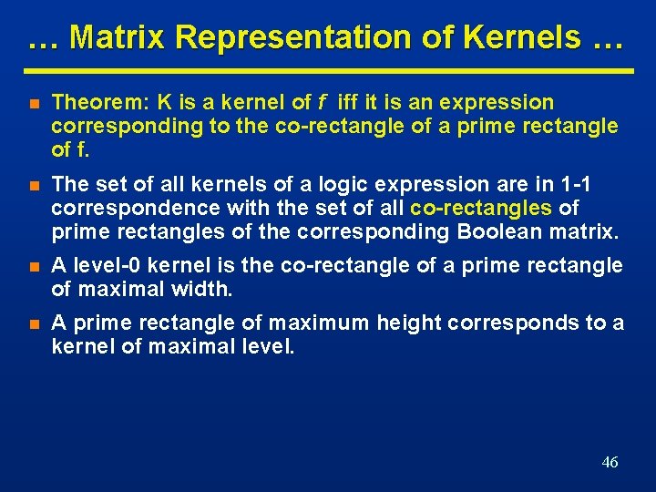
… Matrix Representation of Kernels … n Theorem: K is a kernel of f iff it is an expression corresponding to the co-rectangle of a prime rectangle of f. n The set of all kernels of a logic expression are in 1 -1 correspondence with the set of all co-rectangles of prime rectangles of the corresponding Boolean matrix. n A level-0 kernel is the co-rectangle of a prime rectangle of maximal width. n A prime rectangle of maximum height corresponds to a kernel of maximal level. 46

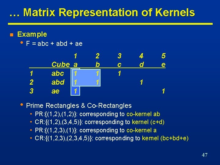
… Matrix Representation of Kernels n Example • F = abc + abd + ae 1 2 3 1 Cube a abc 1 abd 1 ae 1 2 b 1 1 3 c 1 4 d 5 e 1 1 • Prime Rectangles & Co-Rectangles • • PR: {(1, 2), (1, 2)}: corresponding to co-kernel ab CR: {(1, 2), (3, 4, 5)}: corresponding to kernel (c+d) PR: {(1, 2, 3), (1)}: corresponding to co-kernel a CR: {(1, 2, 3), (2, 3, 4, 5)}: corresponding to kernel (bc+bd+e) 47

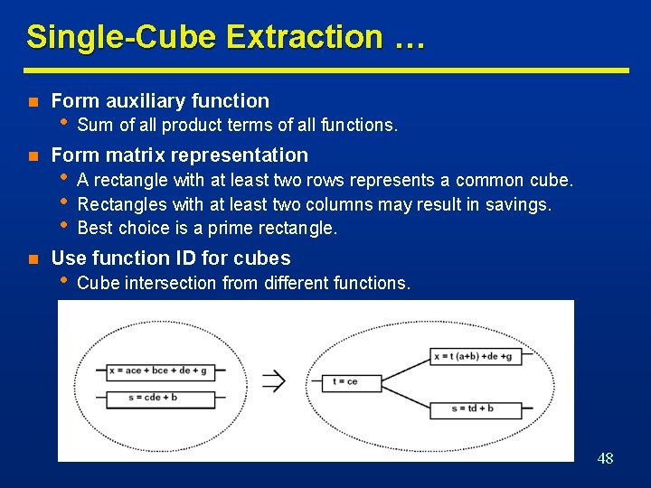
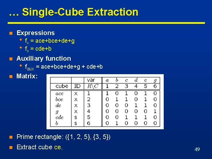
Single-Cube Extraction … n n n Form auxiliary function • Sum of all product terms of all functions. Form matrix representation • • • A rectangle with at least two rows represents a common cube. Rectangles with at least two columns may result in savings. Best choice is a prime rectangle. Use function ID for cubes • Cube intersection from different functions. 48

… Single-Cube Extraction n n Expressions • • fx = ace+bce+de+g fs = cde+b Auxiliary function • faux = ace+bce+de+g + cde+b n Matrix: n Prime rectangle: ({1, 2, 5}, {3, 5}) n Extract cube ce. 49

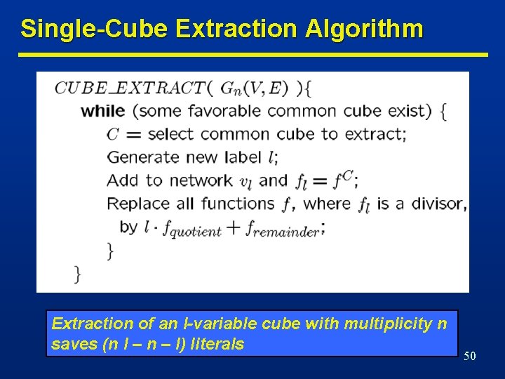
Single-Cube Extraction Algorithm Extraction of an l-variable cube with multiplicity n saves (n l – n – l) literals 50

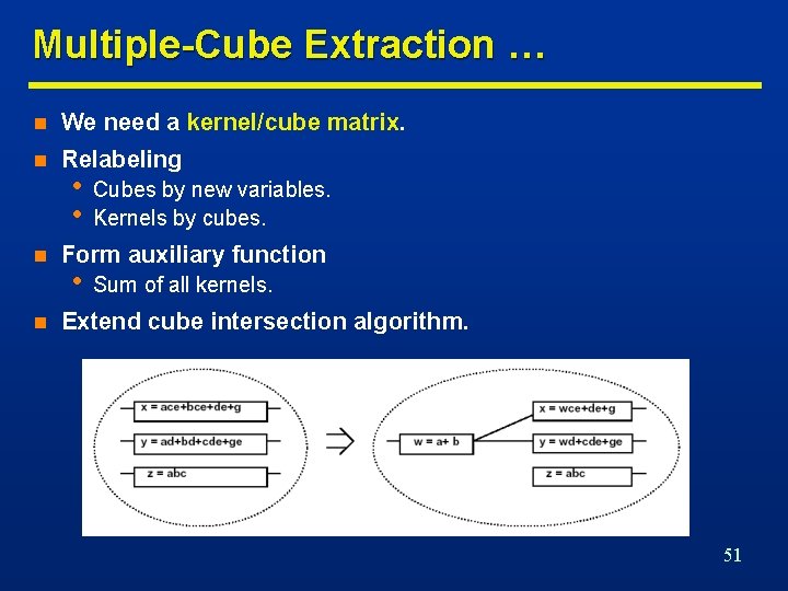
Multiple-Cube Extraction … n We need a kernel/cube matrix. n Relabeling n n • • Cubes by new variables. Kernels by cubes. Form auxiliary function • Sum of all kernels. Extend cube intersection algorithm. 51

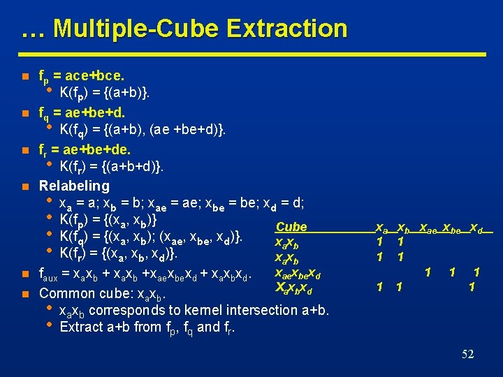
… Multiple-Cube Extraction n n n fp = ace+bce. • K(fp) = {(a+b)}. fq = ae+be+d. • K(fq) = {(a+b), (ae +be+d)}. fr = ae+be+de. • K(fr) = {(a+b+d)}. Relabeling • xa = a; xb = b; xae = ae; xbe = be; xd = d; • K(fp) = {(xa, xb)} Cube • K(fq) = {(xa, xb); (xae, xbe, xd)}. xa xb • K(fr) = {(xa, xb, xd)}. xa xb xaexbexd faux = xaxb +xaexbexd + xaxbxd. X a xbxd Common cube: xaxb. • xaxb corresponds to kernel intersection a+b. • Extract a+b from fp, fq and fr. xa xb xae xbe xd 1 1 1 1 1 52

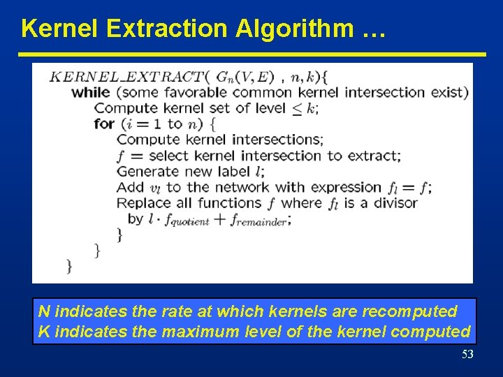
Kernel Extraction Algorithm … N indicates the rate at which kernels are recomputed K indicates the maximum level of the kernel computed 53

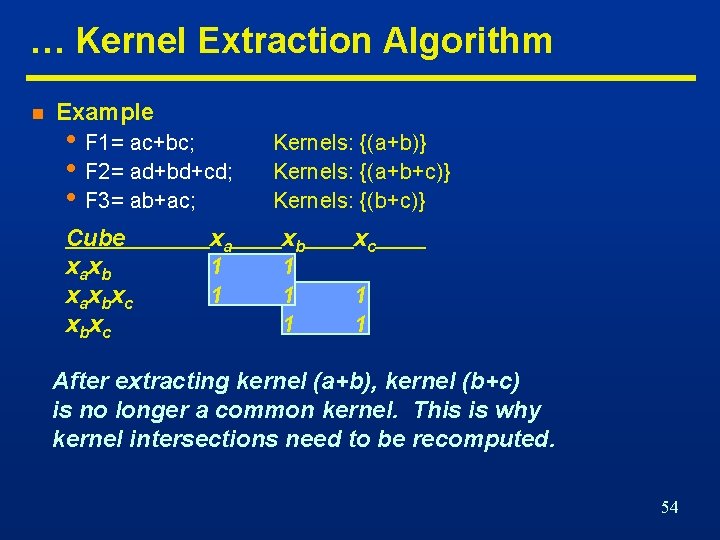
… Kernel Extraction Algorithm n Example • F 1= ac+bc; • F 2= ad+bd+cd; • F 3= ab+ac; Cube x ax b x c xb xc xa 1 1 Kernels: {(a+b)} Kernels: {(a+b+c)} Kernels: {(b+c)} xb 1 1 1 xc 1 1 After extracting kernel (a+b), kernel (b+c) is no longer a common kernel. This is why kernel intersections need to be recomputed. 54

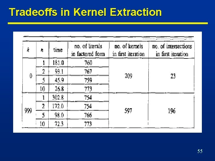
Tradeoffs in Kernel Extraction 55

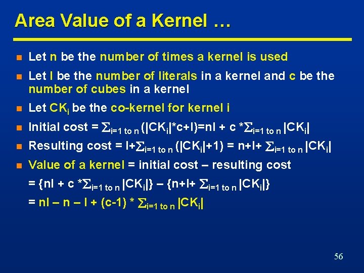
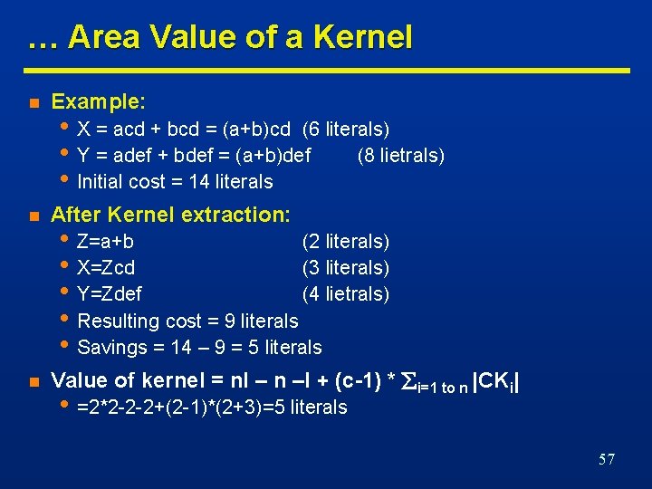
Area Value of a Kernel … n Let n be the number of times a kernel is used n Let l be the number of literals in a kernel and c be the number of cubes in a kernel n Let CKi be the co-kernel for kernel i n Initial cost = i=1 to n (|CKi|*c+l)=nl + c * i=1 to n |CKi| n Resulting cost = l+ i=1 to n (|CKi|+1) = n+l+ i=1 to n |CKi| n Value of a kernel = initial cost – resulting cost = {nl + c * i=1 to n |CKi|} – {n+l+ i=1 to n |CKi|} = nl – n – l + (c-1) * i=1 to n |CKi| 56

… Area Value of a Kernel n Example: n After Kernel extraction: n Value of kernel = nl – n –l + (c-1) * i=1 to n |CKi| • X = acd + bcd = (a+b)cd (6 literals) • Y = adef + bdef = (a+b)def (8 lietrals) • Initial cost = 14 literals • Z=a+b (2 literals) • X=Zcd (3 literals) • Y=Zdef (4 lietrals) • Resulting cost = 9 literals • Savings = 14 – 9 = 5 literals • =2*2 -2 -2+(2 -1)*(2+3)=5 literals 57

Issues in Common Cube and Multiple-Cube Extraction n Greedy approach can be applied in common cube and multiple-cube extraction • Rectangle selection • Matrix update n Greedy approach may be myopic n Non-prime rectangles can contribute to lower cost covers than prime rectangles • Local gain of one extraction considered at a time • Quine’s theorem cannot be applied to rectangles 58

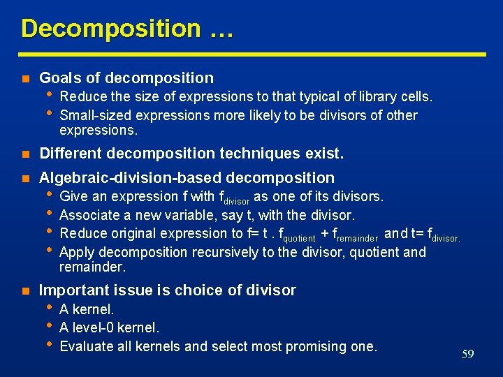
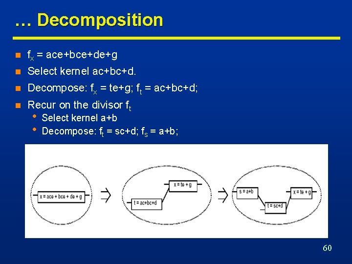
Decomposition … n Goals of decomposition • • Reduce the size of expressions to that typical of library cells. Small-sized expressions more likely to be divisors of other expressions. n Different decomposition techniques exist. n Algebraic-division-based decomposition n • • Give an expression f with fdivisor as one of its divisors. Associate a new variable, say t, with the divisor. Reduce original expression to f= t. fquotient + fremainder and t= fdivisor. Apply decomposition recursively to the divisor, quotient and remainder. Important issue is choice of divisor • • • A kernel. A level-0 kernel. Evaluate all kernels and select most promising one. 59

… Decomposition n fx = ace+bce+de+g n Select kernel ac+bc+d. n Decompose: fx = te+g; ft = ac+bc+d; n Recur on the divisor ft • • Select kernel a+b Decompose: ft = sc+d; fs = a+b; 60

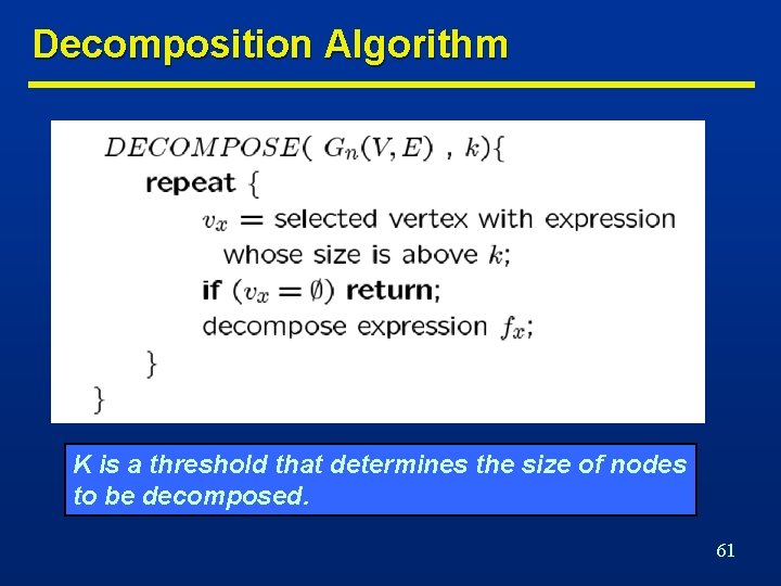
Decomposition Algorithm K is a threshold that determines the size of nodes to be decomposed. 61

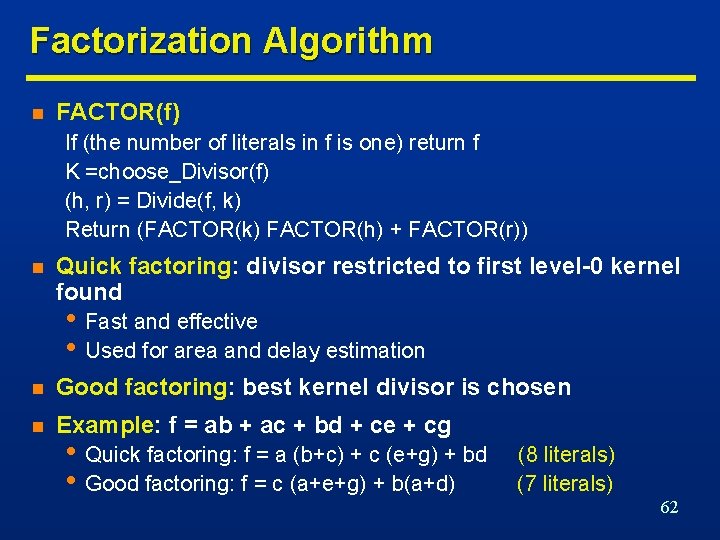
Factorization Algorithm n FACTOR(f) If (the number of literals in f is one) return f K =choose_Divisor(f) (h, r) = Divide(f, k) Return (FACTOR(k) FACTOR(h) + FACTOR(r)) n Quick factoring: divisor restricted to first level-0 kernel found • Fast and effective • Used for area and delay estimation n Good factoring: best kernel divisor is chosen n Example: f = ab + ac + bd + ce + cg • Quick factoring: f = a (b+c) + c (e+g) + bd • Good factoring: f = c (a+e+g) + b(a+d) (8 literals) (7 literals) 62

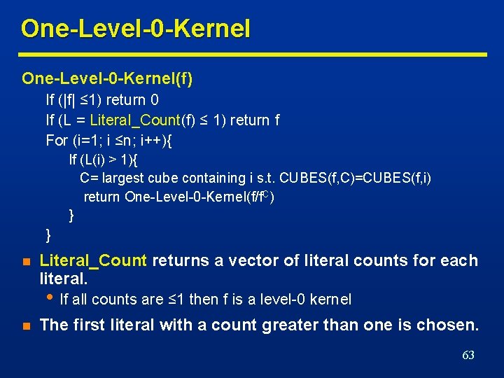
One-Level-0 -Kernel(f) If (|f| ≤ 1) return 0 If (L = Literal_Count(f) ≤ 1) return f For (i=1; i ≤n; i++){ If (L(i) > 1){ C= largest cube containing i s. t. CUBES(f, C)=CUBES(f, i) return One-Level-0 -Kernel(f/f. C) } } n Literal_Count returns a vector of literal counts for each literal. • If all counts are ≤ 1 then f is a level-0 kernel n The first literal with a count greater than one is chosen. 63

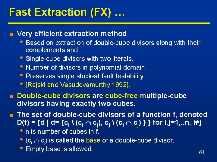
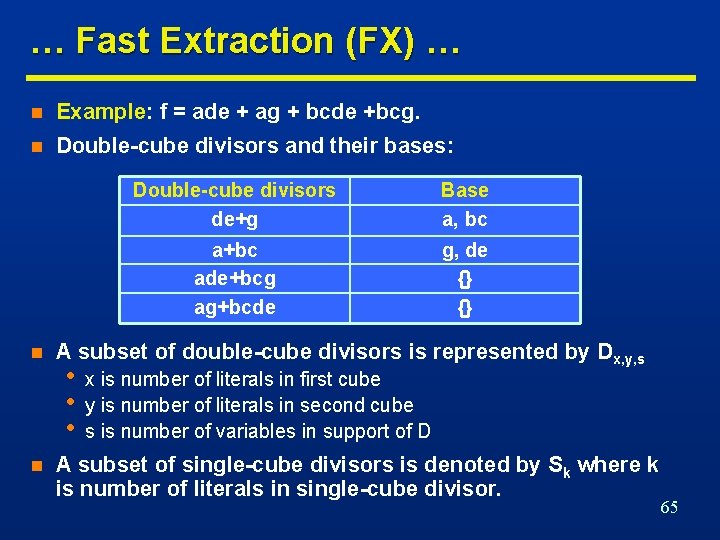
Fast Extraction (FX) … n Very efficient extraction method • Based on extraction of double-cube divisors along with their • • complements and, Single-cube divisors with two literals. Number of divisors in polynomial domain. Preserves single stuck-at fault testability. [Rajski and Vasudevamurthy 1992]. n Double-cube divisors are cube-free multiple-cube divisors having exactly two cubes. n The set of double-cube divisors of a function f, denoted D(f) = {d | d= {ci (ci cj), cj (ci cj) } } for i, j=1, . . n, i≠j • n is number of cubes in f. • (ci cj) is called the base of a double-cube divisor. • Empty base is allowed. 64

… Fast Extraction (FX) … n Example: f = ade + ag + bcde +bcg. n Double-cube divisors and their bases: n n Double-cube divisors de+g Base a, bc a+bc ade+bcg ag+bcde g, de {} {} A subset of double-cube divisors is represented by Dx, y, s • • • x is number of literals in first cube y is number of literals in second cube s is number of variables in support of D A subset of single-cube divisors is denoted by Sk where k is number of literals in single-cube divisor. 65

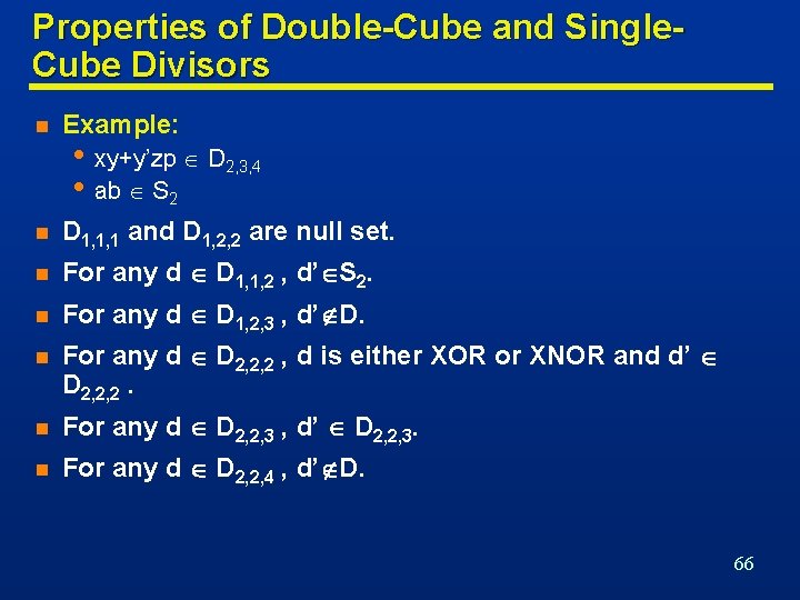
Properties of Double-Cube and Single. Cube Divisors n Example: n D 1, 1, 1 and D 1, 2, 2 are null set. n For any d D 1, 1, 2 , d’ S 2. n For any d D 1, 2, 3 , d’ D. n For any d D 2, 2, 2 , d is either XOR or XNOR and d’ D 2, 2, 2. n For any d D 2, 2, 3 , d’ D 2, 2, 3. n For any d D 2, 2, 4 , d’ D. • xy+y’zp D 2, 3, 4 • ab S 2 66

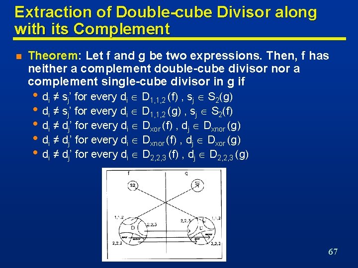
Extraction of Double-cube Divisor along with its Complement n Theorem: Let f and g be two expressions. Then, f has neither a complement double-cube divisor nor a complement single-cube divisor in g if • di ≠ sj’ for every di D 1, 1, 2 (f) , sj S 2(g) • di ≠ sj’ for every di D 1, 1, 2 (g) , sj S 2(f) • di ≠ dj’ for every di Dxor (f) , dj Dxnor (g) • di ≠ dj’ for every di Dxnor (f) , dj Dxor (g) • di ≠ dj’ for every di D 2, 2, 3 (f) , dj D 2, 2, 3 (g) 67

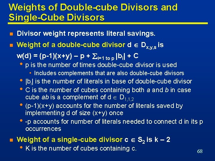
Weights of Double-cube Divisors and Single-Cube Divisors n Divisor weight represents literal savings. n Weight of a double-cube divisor d Dx, y, s is w(d) = (p-1)(x+y) – p + i=1 to p |bi| + C • p is the number of times double-cube divisor is used • Includes complements that are also double-cube divisors • |bi| is the number of literals in base of double-cube divisor • C is the number of cubes containing both a and b in case • • n cube ab is a complement of d D 1, 1, 2 (p-1)(x+y) accounts for the number of literals saved by implementing d of size (x+y) once -p accounts for number of literals needed to connect d in its p occurrences Weight of a single-cube divisor c S 2 is k – 2 • K is the number of cubes containing c. 68

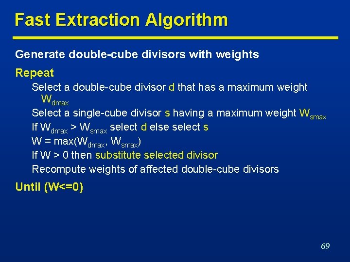
Fast Extraction Algorithm Generate double-cube divisors with weights Repeat Select a double-cube divisor d that has a maximum weight Wdmax Select a single-cube divisor s having a maximum weight Wsmax If Wdmax > Wsmax select d else select s W = max(Wdmax, Wsmax) If W > 0 then substitute selected divisor Recompute weights of affected double-cube divisors Until (W<=0) 69

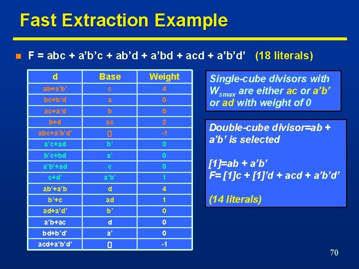
Fast Extraction Example n F = abc + a’b’c + ab’d + a’bd + acd + a’b’d’ (18 literals) d Base Weight ab+a’b’ c 4 bc+b’d a 0 ac+a’d b 0 b+d ac 2 abc+a’b’d’ {} -1 a’c+ad b’ 0 b’c+bd a’ 0 a’b’+ad c 0 c+d’ a’b’ 1 ab’+a’b d 4 b’+c ad 1 ad+a’d’ b’ 0 a’b+ac d 0 bd+b’d’ a’ 0 acd+a’b’d’ {} -1 Single-cube divisors with Wsmax are either ac or a’b’ or ad with weight of 0 Double-cube divisor=ab + a’b’ is selected [1]=ab + a’b’ F= [1]c + [1]’d + acd + a’b’d’ (14 literals) 70

Boolean Methods n Exploit Boolean properties. n Minimization of the local functions. n Slower algorithms, better quality results. n Don’t care conditions related to embedding of a function in an environment • Don't care conditions. • Called external don’t care conditions n External don’t care conditions • Controllability • Observability 71

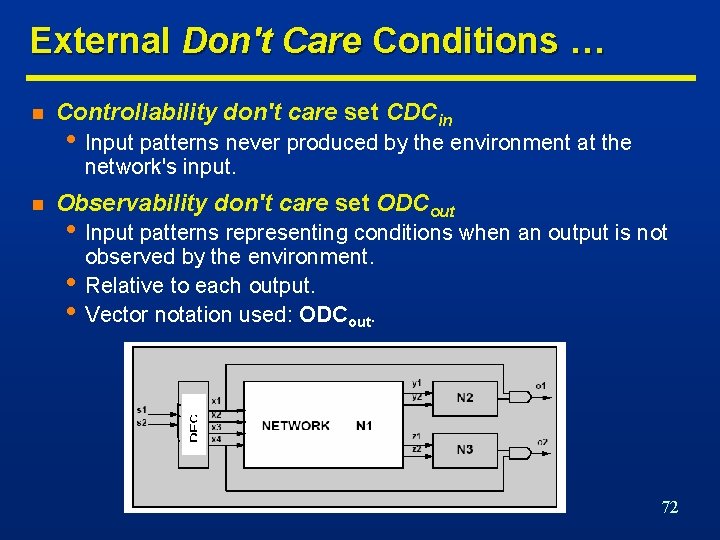
External Don't Care Conditions … n Controllability don't care set CDCin • Input patterns never produced by the environment at the network's input. n Observability don't care set ODCout • Input patterns representing conditions when an output is not • • observed by the environment. Relative to each output. Vector notation used: ODCout. 72

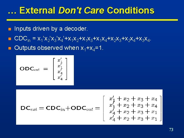
… External Don't Care Conditions n Inputs driven by a decoder. n CDCin = x 1’x 2’x 3’x 4’+x 1 x 2+x 1 x 3+x 1 x 4+x 2 x 3+x 2 x 4+x 3 x 4. n Outputs observed when x 1+x 4=1. 73

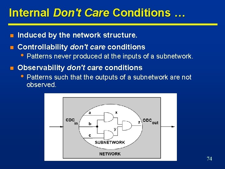
Internal Don't Care Conditions … n Induced by the network structure. n Controllability don't care conditions n Observability don't care conditions • Patterns never produced at the inputs of a subnetwork. • Patterns such that the outputs of a subnetwork are not observed. 74

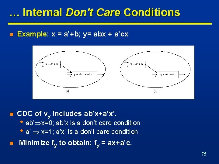
… Internal Don't Care Conditions n Example: x = a’+b; y= abx + a’cx n CDC of vy includes ab’x+a’x’. n • ab’ x=0; ab’x is a don’t care condition • a’ x=1; a’x’ is a don’t care condition Minimize fy to obtain: fy = ax+a’c. 75

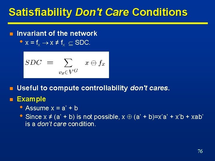
Satisfiability Don't Care Conditions n Invariant of the network • x = f x x ≠ fx SDC. n Useful to compute controllability don't cares. n Example • Assume x = a’ + b • Since x ≠ (a’ + b) is not possible, x (a’ + b)=x’a’ + x’b + xab’ is a don’t care condition. 76

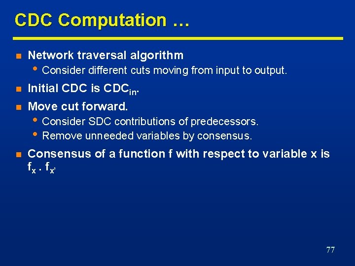
CDC Computation … n Network traversal algorithm n Initial CDC is CDCin. n Move cut forward. n Consensus of a function f with respect to variable x is fx. fx’ • Consider different cuts moving from input to output. • Consider SDC contributions of predecessors. • Remove unneeded variables by consensus. 77

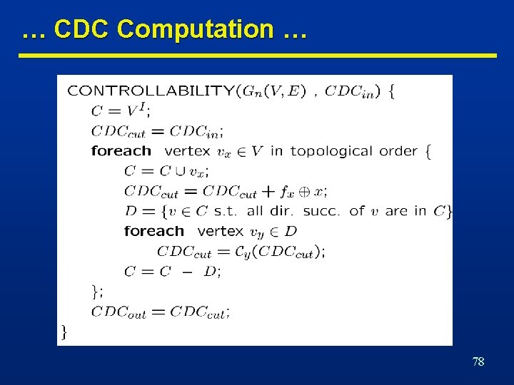
… CDC Computation … 78

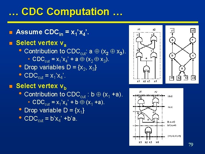
… CDC Computation … n Assume CDCin = x 1’x 4’. n Select vertex va • Contribution to CDCcut: a (x 2 x 3). • CDCcut = x 1’x 4’ + a (x 2 x 3). • Drop variables D = {x 2, x 3} • CDCcut = x 1’x 4’. n Select vertex vb • Contribution to CDCcut : b (x 1 +a). • CDCcut = x 1’x 4’ + b (x 1 +a). • Drop variable D = {x 1} • CDCcut = b’x 4’ +b’a. 79

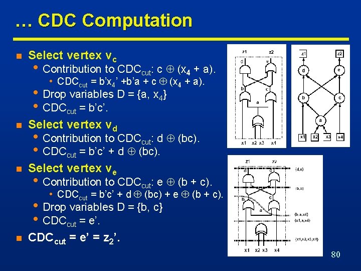
… CDC Computation n Select vertex vc • Contribution to CDCcut: c (x 4 + a). • CDCcut = b’x 4’ +b’a + c (x 4 + a). • Drop variables D = {a, x 4} • CDCcut = b’c’. n Select vertex vd n Select vertex ve • Contribution to CDCcut: d (bc). • CDCcut = b’c’ + d (bc). • Contribution to CDCcut: e (b + c). • CDCcut = b’c’ + d (bc) + e (b + c). • Drop variables D = {b, c} • CDCcut = e’. n CDCcut = e’ = z 2’. 80

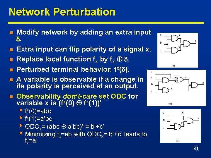
Network Perturbation n n n Modify network by adding an extra input . Extra input can flip polarity of a signal x. Replace local function fx by fx . Perturbed terminal behavior: fx( ). A variable is observable if a change in its polarity is perceived at an output. Observability don’t-care set ODC for variable x is (fx(0) fx(1))’ • fx(0)=abc • fx(1)=a’bc • ODCx= (abc a’bc)’ = b’+c’ • Minimizing fx=ab with ODCx= b’+c’ leads to fx=a. 81

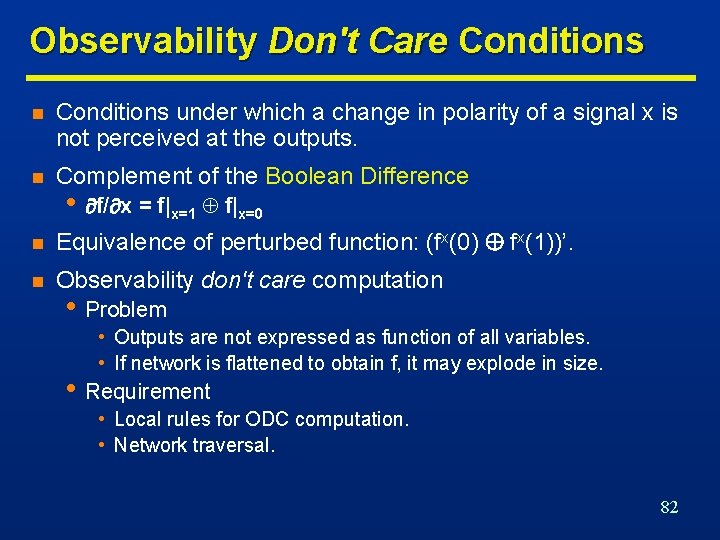
Observability Don't Care Conditions n Conditions under which a change in polarity of a signal x is not perceived at the outputs. n Complement of the Boolean Difference n Equivalence of perturbed function: (fx(0) fx(1))’. n Observability don't care computation • f/ x = f|x=1 f|x=0 • Problem • Outputs are not expressed as function of all variables. • If network is flattened to obtain f, it may explode in size. • Requirement • Local rules for ODC computation. • Network traversal. 82

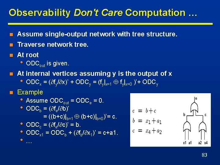
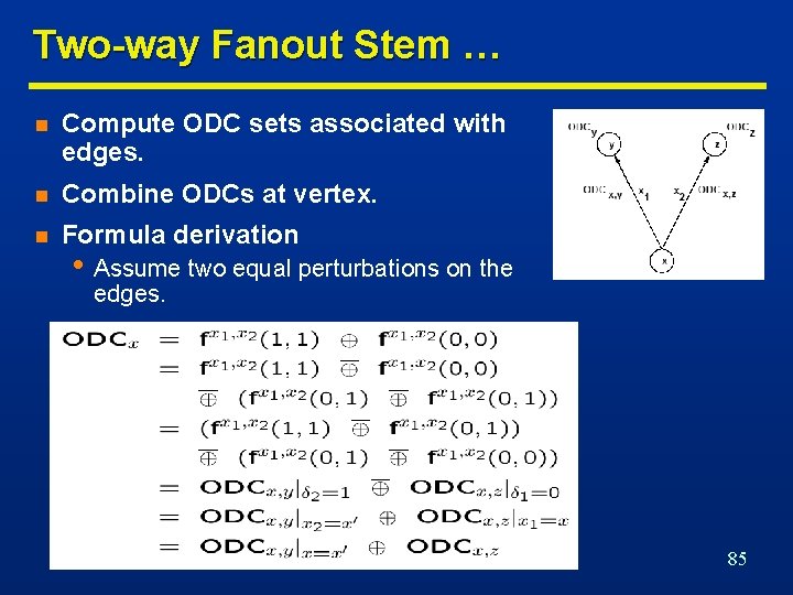
Observability Don't Care Computation … n Assume single-output network with tree structure. n Traverse network tree. n At root n n • ODCout is given. At internal vertices assuming y is the output of x • ODCx = ( fy/ x)’ + ODCy = (fy|x=1 fy|x=0 )’+ ODCy Example • • • Assume ODCout = ODCe = 0. ODCb = ( fe/ b)’ = ((b+c)|b=1 (b+c)|b=0)’= c. ODCc = ( fe/ c)’ = b. ODCx 1 = ODCb + ( fb/ x 1)’ = c+a 1. … 83

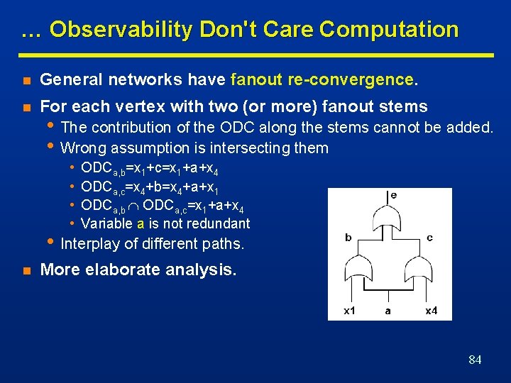
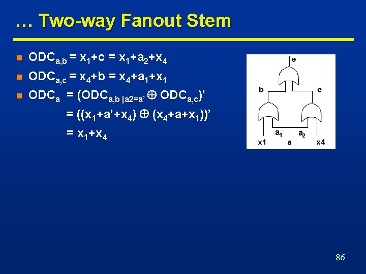
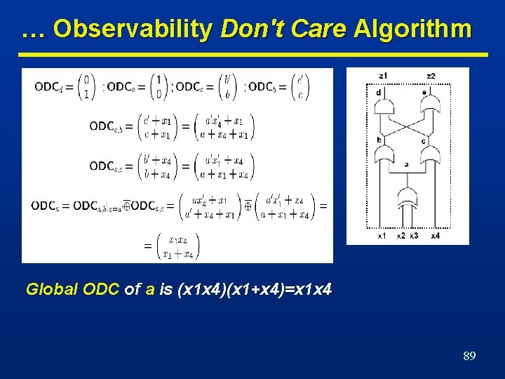
… Observability Don't Care Computation n General networks have fanout re-convergence. n For each vertex with two (or more) fanout stems • The contribution of the ODC along the stems cannot be added. • Wrong assumption is intersecting them • • ODCa, b=x 1+c=x 1+a+x 4 ODCa, c=x 4+b=x 4+a+x 1 ODCa, b ODCa, c=x 1+a+x 4 Variable a is not redundant • Interplay of different paths. n More elaborate analysis. 84

Two-way Fanout Stem … n Compute ODC sets associated with edges. n Combine ODCs at vertex. n Formula derivation • Assume two equal perturbations on the edges. 85

… Two-way Fanout Stem n ODCa, b = x 1+c = x 1+a 2+x 4 n ODCa, c = x 4+b = x 4+a 1+x 1 n ODCa = (ODCa, b |a 2=a’ ODCa, c)’ = ((x 1+a’+x 4) (x 4+a+x 1))’ = x 1+x 4 a 1 a 2 86

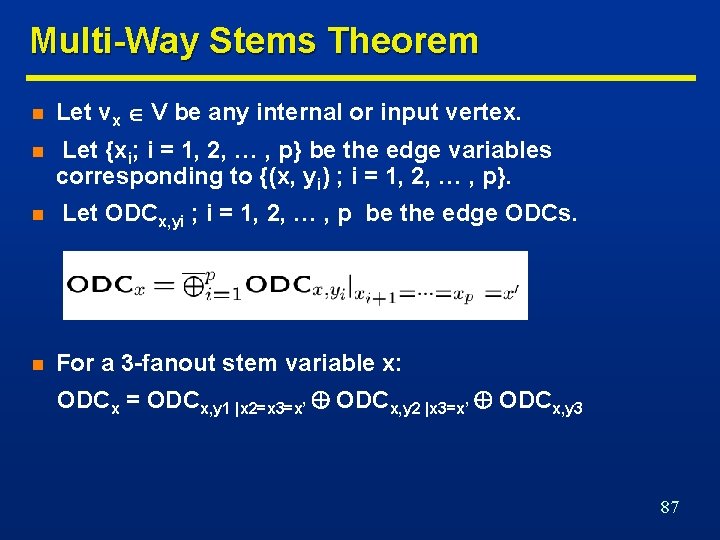
Multi-Way Stems Theorem n Let vx V be any internal or input vertex. n Let {xi; i = 1, 2, … , p} be the edge variables corresponding to {(x, yi) ; i = 1, 2, … , p}. n n Let ODCx, yi ; i = 1, 2, … , p be the edge ODCs. For a 3 -fanout stem variable x: ODCx = ODCx, y 1 |x 2=x 3=x’ ODCx, y 2 |x 3=x’ ODCx, y 3 87

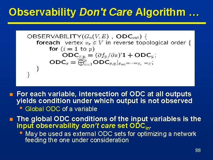
Observability Don't Care Algorithm … n For each variable, intersection of ODC at all outputs yields condition under which output is not observed • Global ODC of a variable n The global ODC conditions of the input variables is the input observability don’t care set ODCin. • May be used as external ODC sets for optimizing a network feeding the one under consideration 88

… Observability Don't Care Algorithm Global ODC of a is (x 1 x 4)(x 1+x 4)=x 1 x 4 89

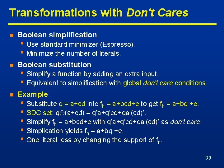
Transformations with Don't Cares n Boolean simplification n Boolean substitution n Example • Use standard minimizer (Espresso). • Minimize the number of literals. • Simplify a function by adding an extra input. • Equivalent to simplification with global don't care conditions. • Substitute q = a+cd into fh = a+bcd+e to get fh = a+bq +e. • SDC set: q (a+cd) = q’a+q’cd+qa’(cd)’. • Simplify fh = a+bcd+e with q’a+q’cd+qa’(cd)’ as don't care. • Simplication yields fh = a+bq +e. • One literal less by changing the support of fh. 90

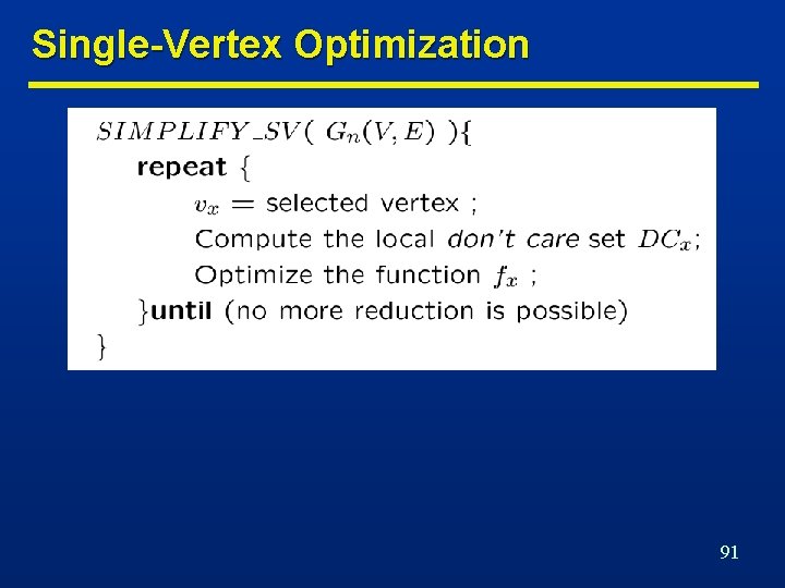
Single-Vertex Optimization 91

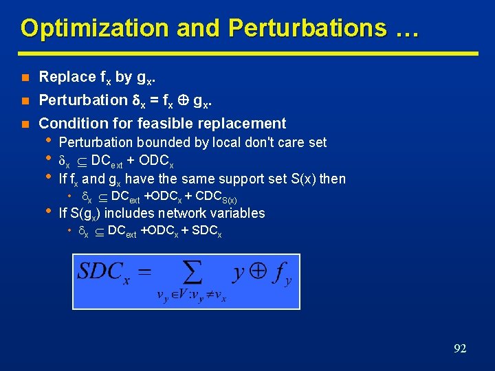
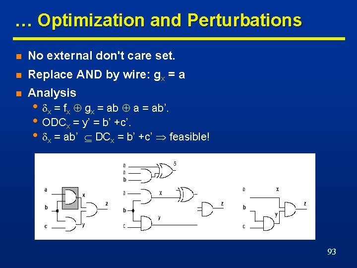
Optimization and Perturbations … n Replace fx by gx. n Perturbation x = fx gx. n Condition for feasible replacement • • • Perturbation bounded by local don't care set x DCext + ODCx If fx and gx have the same support set S(x) then • If S(gx) includes network variables • x DCext +ODCx + CDCS(x) • x DCext +ODCx + SDCx 92

… Optimization and Perturbations n No external don't care set. n Replace AND by wire: gx = a n Analysis • x = fx gx = ab a = ab’. • ODCx = y’ = b’ +c’. • x = ab’ DCx = b’ +c’ feasible! 93

Synthesis and Testability n Assumptions n Full testability n Synergy between synthesis and testing. n Testable networks correlate to small-area networks. n Don't care conditions play a major role. • Ease of testing a circuit. • Combinational circuit. • Single or multiple stuck-at faults. • Possible to generate test set for all faults. 94

Test for Stuck-at-Faults n Net y stuck-at 0 • Input pattern that sets y to true. • Observe output. • Output of faulty circuit differs. • {t | y(t). ODC’y(t) = 1}. n Net y stuck-at 1 n Need controllability and observability. • Same, but set y to false. • {t | y’(t). ODC’y(t) = 1}. 95

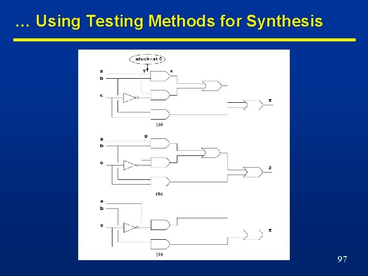
Using Testing Methods for Synthesis … n Redundancy removal. • Use ATPG to search for untestable faults. n If stuck-at 0 on net y is untestable n If stuck-at 1 on y is untestable • Set y = 0. • Propagate constant. • Set y = 1. • Propagate constant. 96

… Using Testing Methods for Synthesis 97

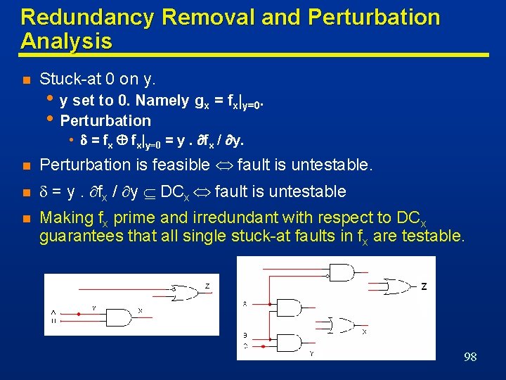
Redundancy Removal and Perturbation Analysis n Stuck-at 0 on y. • y set to 0. Namely gx = fx|y=0. • Perturbation • = fx fx|y=0 = y. fx / y. n Perturbation is feasible fault is untestable. n = y. fx / y DCx fault is untestable n Making fx prime and irredundant with respect to DCx guarantees that all single stuck-at faults in fx are testable. 98

Synthesis for Testability n Synthesize networks that are fully testable. n Two-level forms • Single stuck-at faults. • Multiple stuck-at faults. • Full testability for single stuck-at faults • Prime and irredundant cover. • Full testability for multiple stuck-at faults • Prime and irredundant cover when • Single-output function. • No product term sharing in case of multiple outputs i. e. each output is prime and irredundant. 99

… Synthesis for Testability n A complete single-stuck-at fault test set for a singleoutput sum-of-product circuit is a complete test set for all multiple stuck-at faults. n Single stuck-at fault testability of multiple-level network does not imply multiple stuck-at fault testability. n Fast extraction transformations are single stuck-at fault test-set preserving transformations. n Algebraic transformations preserve multiple stuck-at fault testability but not single stuck-at fault testability • Factorization • Substitution (without complement) • Cube and kernel extraction 100

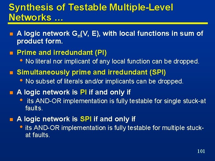
Synthesis of Testable Multiple-Level Networks … n A logic network Gn(V, E), with local functions in sum of product form. n Prime and irredundant (PI) n Simultaneously prime and irredundant (SPI) n A logic network is PI if and only if n • No literal nor implicant of any local function can be dropped. • No subset of literals and/or implicants can be dropped. • its AND-OR implementation is fully testable for single stuck-at faults. A logic network is SPI if and only if • its AND-OR implementation is fully testable for multiple stuckat faults. 101

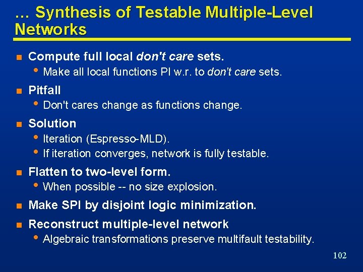
… Synthesis of Testable Multiple-Level Networks n Compute full local don't care sets. n Pitfall n Solution n Flatten to two-level form. n Make SPI by disjoint logic minimization. n Reconstruct multiple-level network • Make all local functions PI w. r. to don't care sets. • Don't cares change as functions change. • Iteration (Espresso-MLD). • If iteration converges, network is fully testable. • When possible -- no size explosion. • Algebraic transformations preserve multifault testability. 102

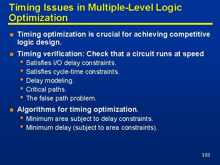
Timing Issues in Multiple-Level Logic Optimization n Timing optimization is crucial for achieving competitive logic design. n Timing verification: Check that a circuit runs at speed n Algorithms for timing optimization. • Satisfies I/O delay constraints. • Satisfies cycle-time constraints. • Delay modeling. • Critical paths. • The false path problem. • Minimum area subject to delay constraints. • Minimum delay (subject to area constraints). 103

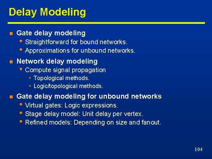
Delay Modeling n Gate delay modeling n Network delay modeling • Straightforward for bound networks. • Approximations for unbound networks. • Compute signal propagation • Topological methods. • Logic/topological methods. n Gate delay modeling for unbound networks • Virtual gates: Logic expressions. • Stage delay model: Unit delay per vertex. • Refined models: Depending on size and fanout. 104

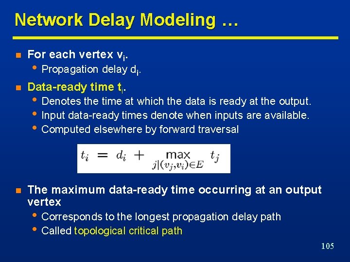
Network Delay Modeling … n For each vertex vi. n Data-ready time ti. n The maximum data-ready time occurring at an output vertex • Propagation delay di. • Denotes the time at which the data is ready at the output. • Input data-ready times denote when inputs are available. • Computed elsewhere by forward traversal • Corresponds to the longest propagation delay path • Called topological critical path 105

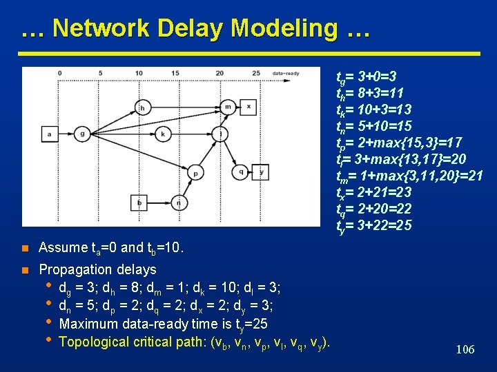
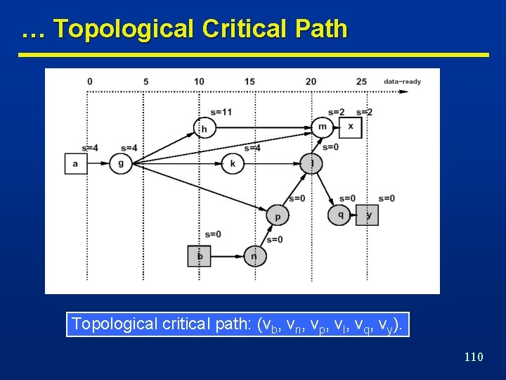
… Network Delay Modeling … tg= 3+0=3 th= 8+3=11 tk= 10+3=13 tn= 5+10=15 tp= 2+max{15, 3}=17 tl= 3+max{13, 17}=20 tm= 1+max{3, 11, 20}=21 tx= 2+21=23 tq= 2+20=22 ty= 3+22=25 n Assume ta=0 and tb=10. n Propagation delays • dg = 3; dh = 8; dm = 1; dk = 10; dl = 3; • dn = 5; dp = 2; dq = 2; dx = 2; dy = 3; • Maximum data-ready time is ty=25 • Topological critical path: (vb, vn, vp, vl, vq, vy). 106

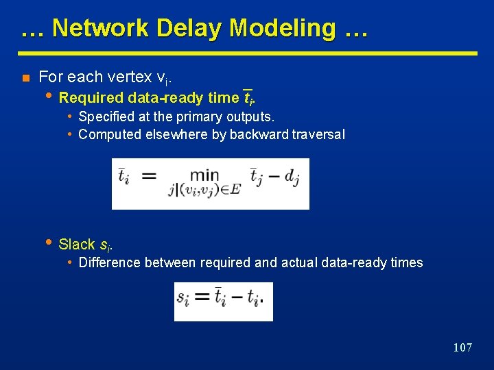
… Network Delay Modeling … n For each vertex vi. • Required data-ready time ti. • Specified at the primary outputs. • Computed elsewhere by backward traversal • Slack si. • Difference between required and actual data-ready times 107

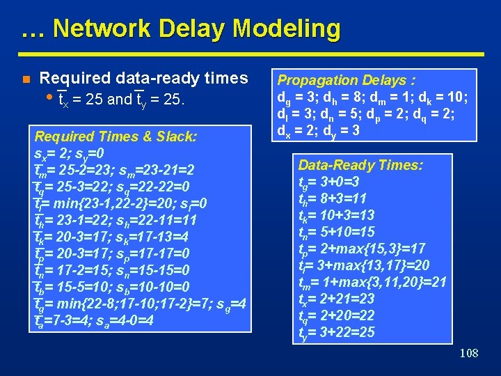
… Network Delay Modeling n Required data-ready times • tx = 25 and ty = 25. Required Times & Slack: sx= 2; sy=0 tm= 25 -2=23; sm=23 -21=2 tq= 25 -3=22; sq=22 -22=0 tl= min{23 -1, 22 -2}=20; sl=0 th= 23 -1=22; sh=22 -11=11 tk= 20 -3=17; sk=17 -13=4 tp= 20 -3=17; sp=17 -17=0 tn= 17 -2=15; sn=15 -15=0 tb= 15 -5=10; sb=10 -10=0 tg= min{22 -8; 17 -10; 17 -2}=7; sg=4 ta=7 -3=4; sa=4 -0=4 Propagation Delays : dg = 3; dh = 8; dm = 1; dk = 10; dl = 3; dn = 5; dp = 2; dq = 2; dx = 2; dy = 3 Data-Ready Times: tg= 3+0=3 th= 8+3=11 tk= 10+3=13 tn= 5+10=15 tp= 2+max{15, 3}=17 tl= 3+max{13, 17}=20 tm= 1+max{3, 11, 20}=21 tx= 2+21=23 tq= 2+20=22 ty= 3+22=25 108

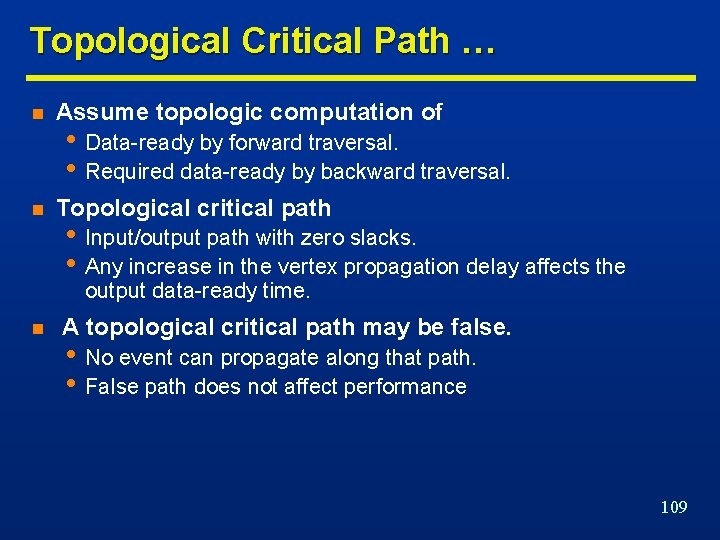
Topological Critical Path … n Assume topologic computation of n Topological critical path • Data-ready by forward traversal. • Required data-ready by backward traversal. • Input/output path with zero slacks. • Any increase in the vertex propagation delay affects the output data-ready time. n A topological critical path may be false. • No event can propagate along that path. • False path does not affect performance 109

… Topological Critical Path Topological critical path: (vb, vn, vp, vl, vq, vy). 110

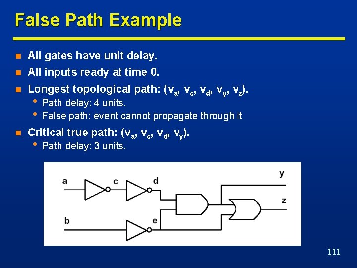
False Path Example n All gates have unit delay. n All inputs ready at time 0. n Longest topological path: (va, vc, vd, vy, vz). n • • Path delay: 4 units. False path: event cannot propagate through it Critical true path: (va, vc, vd, vy). • Path delay: 3 units. 111

Algorithms for Delay Minimization … n n n Alternate • • Critical path computation. Logic transformation on critical vertices. Consider quasi critical paths • • Paths with near-critical delay. Small slacks. Small difference between critical paths and largest delay of a non-critical path leads to smaller gain in speeding up critical paths only. 112

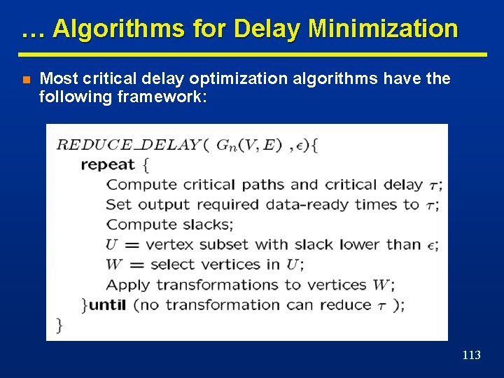
… Algorithms for Delay Minimization n Most critical delay optimization algorithms have the following framework: 113

Transformations for Delay Reduction … n Reduce propagation delay. n Reduce dependencies from critical inputs. n Favorable transformation • Reduces local data-ready time. • Any data-ready time increase at other vertices is bounded by the local slack. n Example • Unit gate delay. • Transformation: Elimination. • Always favorable. • Obtain several area/delay trade-off points. 114

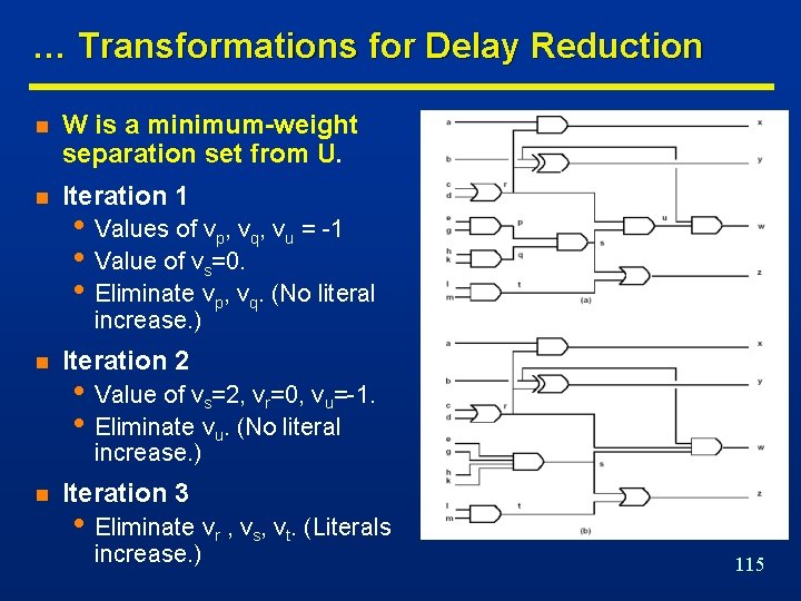
… Transformations for Delay Reduction n W is a minimum-weight separation set from U. n Iteration 1 • Values of vp, vq, vu = -1 • Value of vs=0. • Eliminate vp, vq. (No literal increase. ) n Iteration 2 • Value of vs=2, vr=0, vu=-1. • Eliminate vu. (No literal increase. ) n Iteration 3 • Eliminate vr , vs, vt. (Literals increase. ) 115

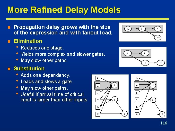
More Refined Delay Models n Propagation delay grows with the size of the expression and with fanout load. n Elimination n • • • Reduces one stage. Yields more complex and slower gates. May slow other paths. Substitution • • Adds one dependency. Loads and slows a gate. May slow other paths. Useful if arrival time of critical input is larger than other inputs 116

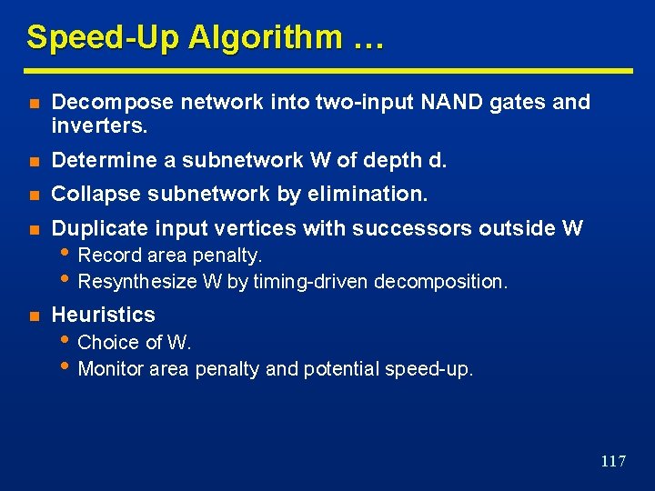
Speed-Up Algorithm … n Decompose network into two-input NAND gates and inverters. n Determine a subnetwork W of depth d. n Collapse subnetwork by elimination. n Duplicate input vertices with successors outside W n Heuristics • Record area penalty. • Resynthesize W by timing-driven decomposition. • Choice of W. • Monitor area penalty and potential speed-up. 117

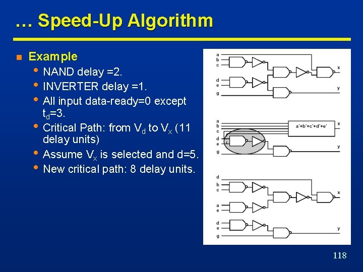
… Speed-Up Algorithm n Example • NAND delay =2. • INVERTER delay =1. • All input data-ready=0 except • • • td=3. Critical Path: from Vd to Vx (11 delay units) Assume Vx is selected and d=5. New critical path: 8 delay units. 118