Logic and Logic Programming Logic Propositional Logic First

Logic and Logic Programming

Logic • Propositional Logic • First Order Predicate Logic

Propositions • A proposition is a declarative sentence. • e. g. Woff is a dog. • e. g. Jim is the husband of Mary. • A proposition is represented by a logical symbol. • P: Woff is a dog. • R: Jim is the husband of Mary.

Sentences • True and False are both logical constants. • Logical constants are sentences. • e. g. True is a propositional logic sentence. • Logical symbols are sentences. • e. g. P is a propositional logic sentence.

Logical Connectives • Logical Connectives are • Ù (and) • Ú (or) • Þ (implication) • Û (bi-conditional) • Negation • Ø (not)

Formal Grammar • Sentence : : = Atomic. Sentence | Complex. Sentence • Atomic. Sentence : : = True | False | P | Q | … • Complex. Sentence : : = (Sentence) | Sentence Connective Sentence | ØSentence • Connective : : = Ù | Ú | Þ | Û

Truth Values • P Q ØP P Ù Q P Ú Q P Þ Q P Û Q • • F F T T T F F F T T T F F T

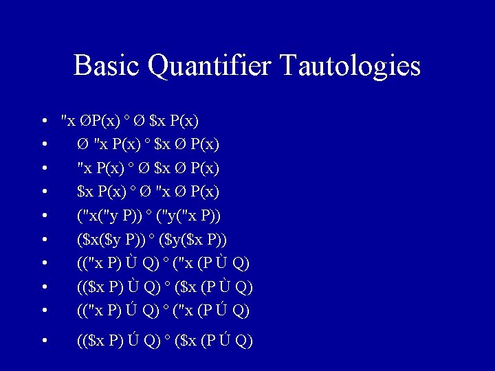
Validity • A sentence is valid if and only if it is true under all possible interpretations in all possible worlds. (Russell, AI: a modern approach) • Valid sentences are also called tautologies.

Some Useful Tautologies • • • Ø(P Ù Q) Û ØP Ú ØQ Ø(P Ú Q) Û ØP Ù ØQ P Þ Q Û ØP Ú Q P Ù Ø P Û False True Þ Q Û Q

Some Inference Rules • • • Modus Pones P Þ Q, P Q Syllogism P Þ Q, Q Þ R PÞR

Horn Clauses • A Horn Clause is a sentence in the following form • P 1 Ù P 2 Ù … Ù Pn Þ Q • Prolog only works with logical sentences which are Horn Clauses

First Order Predicate Logic • Allows the following to be modeled • objects • properties of objects • relations among the objects • Like propositional logic, FOL has sentences • Additionally it has terms which allow the representation of objects

Terms • A term is a logical expression which refers to an object. (Russel, 188) • Elements of a term • Constant Symbols - A, B, John • Predicate Symbols - refer to a relation • Function Symbols - refer to a relation which is a function

Sentences • Atomic Sentences - state a fact • e. g. company(gordon). • e. g. location(gordon, usa) • Complex Sentences - formed from: • atomic sentences • logical connectives • quantifiers

Quantifiers • Universal Quantifier (") • "x is read “For all x …” • All cats are mammals. • "x (Cat(x) Þ Mammal(x)) • Extensile Quantifier ($) • $x is read “There exists an x. . ” • Spot has a sister who is a cat. • $x ( Sister(x, Spot) Ù Cat(x))

Other Paradigms : Logic Programming refers loosely to • The use of facts and rules to represent information. • The use of deduction to answer queries. An Example of a rule is overlap(X, Y) : - member(M, X), member(M, Y) Here lists X and Y overlap if there is some member M that is a member of both X and Y. In order to deduce this we need Prolog to answer queries.

How Prolog came into Existence ? • The concept of logic programming is linked historically to Prolog (Programming Logic). • Prolog was first applied to natural language Processing. Later it has been used for specifying algorithms, searching databases, writing compilers. It can do all applications for which Lisp might be used. • Prolog is effective for applications involving pattern matching, backtrack searching or incomplete information. • In short, labor in Logic Programming is denoted by algorithm = logic + control We supply logic part, Prog. Lang supplies control part.

Prolog has various dialects, Here we will talk about Edinburgh Prolog. Control In Edinburgh Prolog proceeds from left to right. The rule: P if Q 1 and Q 2 and …. And Qk. K>= 0 can be read as to deduce P, deduce Q 1, deduce Q 2 …. Deduce Qk Computing with Relations : • Logic Programming deals with relations rather than functions. It is based on the premise that programming with relations is more flexible than with functions. • Prolog deals with lists. Lists are written between brackets [ and ] , so [ ] is an empty list. [b, c] is a list with two symbols b and c. here b is head and c is tail.

Relations : • Relation append is a set of tuples of the form (X, Y, Z) where Z consists of elements of X followed by elements of Y. • Relations are specified by rules written in pseudo code as P if Q 1 and Q 2 and …. And Qk. K>= 0. Such rules are called as Horn clauses. • A fact is a special case of rule, in which k = 0 and P holds without any conditions, written simply as P Rules append( x, y, z) ----> append x and y to get z. append( [ ], y, y ) ----> append [ ] and y to get y.

Queries : Logic Prog. is driven by queries about relations. Horn clauses cannot represent negative information, Hence queries are answered as yes / fail rather than yes / no answers. ? - append( [a, b], [c, d], [a, b, c, d] ) ----> Yes ? - append( [a, b], [c, d], Z ) ----> Yes when Z = [a, b, c, d] ? - append( [a, b], Y, [a, b, c, d]) ----> Yes when Y = [c, d] ? - append( X, [c, d], [a, b, c, d]) ----> Yes when X = [a, b] ? - append( X, [d, c], [a, b, c, d]) ----> Fail Informally, Relations has no sense of direction, no prejudice who is computed from whom. Relations treat arguments and results uniformly.

Introduction To Prolog : • Facts, rules and queries are specified using terms. Facts, rules, queries number : 0 , 1972 variable : X, Source atom : lisp, algol 60 TERMS Simple Term Compound Term atom(subterms) link(bcpl, c)

Introduction to Prolog • Prolog is a logic programming language • Prolog is based upon First Order Logic (FOL) • A Prolog program consists of a Knowledge Base composed of: • facts • rules • All facts and rules must be expressed as Horn Clauses

Syntax Rules • Predicates (functors) must start with lowercase letter. • Constants begin with a lower-case letter or number. • Variables begin with an upper-case letter or an (_). • All sentences (clauses) must end with a period.

Clauses • • • All clauses have a head and a body. head : - body. The symbol : - is read if

Facts • A fact is stated as a functor using constants. • e. g. dog(woff). • A fact has only a head • A fact may be a functor without an argument list. • A single constant. • e. g. woff.

Rules • A rule has both head and body • dog(X) : - barks(X), wags_tail(X) • head is: dog(X) • body is: barks(X), wags_tail(X) • FOL form: if body then head • "X (barks(X) Ù wags_tain(X) Þ dog(X))

A Prolog Program • Knowledge Base • dog(X) : - barks(X), wags_tail(X)barks(woff)barks(spot)wags_tail( woff) • Queries • ? - dog(woff) => yes • ? - dog(spot) => no • Means no more matches found.

Using Variables • Knowledge Base • dog(X) : - barks(X), wags_tail(X)barks(woff)barks(spot)wags_ta il(woff) • Query • ? - dog(Y) => Y = woff

Prolog’s Search Algorithm • Prolog uses a goal directed search of the KB • Depth first search is used • Query clauses are used as goals and searched left to right • KB clauses are searched in the order they occur in the KB • Goals are matched to the head of clauses • Terms must unify based upon variable substitution before they match

Unification • Idea substitute terms for variables so that facts that match a predicate with a variable can be found. • A substitution is a function from variables to terms. • {V ® [a, b], Y® [a, b, c]} is a substitution. • Y {V ® [a, b], Y® [a, b, c]} = [a, b, c]

Facts and Rules in file links : link(fortran, algol 60) link(algol 60, cpl) link(cpl, bcpl) link(bcpl, c) link(c, c++) link(algol 60, simula 67) link(simula 67, c++) link(simula 67, smalltalk 80) Queries are also called goals. ? - link(cpl, bcpl) , link(bcpl, c) -----> yes

? - link(algol 60, L) and link(L, M)? A solution to query is a binding of variable to makes the query true. A query with solution is satisfiable. The system responds to a satisfiable query. L = cpl , M = bcpl ; L = simula 67 , M = c++ ; L = simula 67 , M = smalltalk 80 ; Universal Facts and Rules : A rule <term> : - <term>1, <term>2, ……<term>k head conditions

A fact is a special case of a rule. A fact has no head and conditions. path(L, L) ---> fact. We take a path of zero links to be from L to itself. Path(L, M) : - link(L, X), path(X, M) A path from L to M begins with a link to some X and continues along the path from X to M. Unification : Deduction in Prolog is based on concept of unification. ? - f(X, b) = f(a, Y) Here, f(a, b) is an instance of f(X, b) because it is obtained by substituting subterm ‘a’ for variable X in f(X, b). Similarly

f(a, b) is an instance of f(a, Y) because it is obtained by replacing subterm ‘b’ for variable Y in f(a, Y) X=a Y=b For Example, g(a, a) is an instance of g(x, x). However, g(a, b) is not an instance of g(x, x) because we cannot substitute ‘a’ for one occurrence of x and ‘b’ for another occurrence of x. Arithmetic • X = 2+3 ---> simply binds variable X to term 2+3 • X is 2+3 ---> The Infix operator evaluates expression and binds 5 to X.

? - X is 2+3 , X = 5 yes ? - X is 2+3 , X = 2+3 no fails because 2+3 does not unify with 5. Term 2+3 is the application of operator + to the arguments 2 and 3, whereas 5 is simply the integer 5. Hence, 2+3 does not unify with 5. Data Structures In Prolog supports several notations for writing Lisp-like lists. They sweeten the syntax without adding any new capabilities.

Lists in Prolog : • The simplest way to write a list is to enumerate its elements • The list containing three atoms a, b and c is written as [a, b, c] • Empty List is written as [ ] • Unification can be used to extract the components of a list. for example : ? - [H | T] = [a, b, c] ---> H = a , T = [b, c]. • In Prolog any tree can be written as term, any term can be written as tree. Example : Term node (K, S, T) can be represented as tree.

K S T • Let atom empty represent binary search tree (K, S, T) with an integer value K at the root, left subtree S, and right subtree T. Terms for representing Binary trees leaf nonleaf(leaf, leaf)

nonleaf(leaf, leaf), nonleaf(leaf, leaf) Member(k, node(k, _, _ ) represent a binary search tree with k at the root and some unnamed left and right subtrees. Beyond trees, variables in Prolog allow terms to represent data structures with sharing. Terms can also represent graphs with cycles.

5. 4 Programming Techniques How does Prolog process queries ? -by backtracking and unification backtracking unification - find solution if exist - place holder variable gets filled in later with value

Guess and Verify Query query: conclusion if guess(…, S, …) and verify(…, S, …); ? - conclusion( ) : - guess( ) , verify( ) find solution to guess( ) and match them against verify( ). If match then conclusion( ).

Example: ? - overlap(X, Y) : - member(M, X) , member(M, Y) find M from list X, and verify M also appears in list Y. If so, then overlap(X, Y).

Prolog processes from left to right. - Watch out for efficiency and unexpected. example: ? - X = [1, 2, 3] , member(a, X). X is a list of [1, 2, 3]. Is ‘a’ a member of X ? ? - member(a, X) , X = [1, 2, 3]. find all solution where a is member of X. ‘a’ can be anywhere in X, so finds infinite possibilities for a, but doesn’t find match in X.

Variable as place holders. open list - list with variable at end closed list - no variable at end Example: [ a, b | X ] ==> open list [ a , b ] ==> closed list

Prolog uses machine generated variables to represent variable at the end of list. Uses underscore + integer. example: ? - L = [ a , b | X ] L = [ a , b | _1] X = _1 variable _1 now corresponds to end marker X

Expand on previous example: ? - L = [ a , b | X ] , X = [ c , Y ] X = _1 L = [ a , b | _1 ] X = _1 = [ c , Y ] = [ c | _2 ] L = [ a , b | _1] = [ a , b | [ c | 2 ] ] = [ a , b , c | _2] _1 unifies with [ c | _2 ] -- like assignment

Example: Queue Manipulation enter( a, Q , R ) ==> when element ‘a’ enters queue Q, we get queue R leave( a , Q , R ) ==> when element ‘a’ leaves queue Q, we get queue R in queue q( L, E ) L = open list E = end marker ( some suffix of L ) content = elements of L, but not in E

Queue Manipulation Cont. Rules: setup( q( X , X ) ). enter( A , q( X , Y ) , q( X , Z ) : - Y = [ A | Z ]. leave( A , q( X , Z ) , q( X , Y ) : - Y = [ A | Y ]. wrapup( q( [ ] , [ ] ) ). What do these mean ?

setup( q( X , X ) ) returns q( open list , end marker ) Example: ? - setup( Q ) Q = q( X , X ) Q = q( _1 , _1 )

enter( A , q ( X, Y) , q(X, Z) ) : - Y = [A | Z]. In plain English: To enter element ‘A’ into queue q( X, Y) bind/unify/assign Y to list [ A | Z ] where Z is new end marker, and return resulting query q( X, Z)

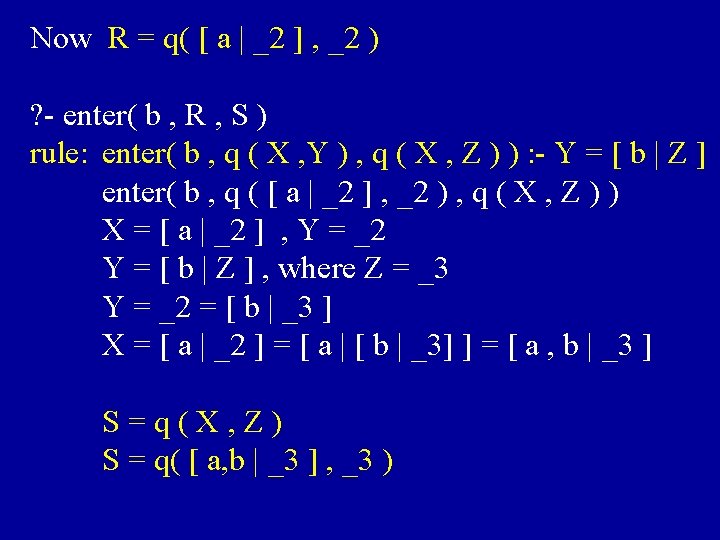
Example: ? - setup(Q) Q = q( X , X ) Q = q( _1 , _1 ) ? - enter( a , Q , R ) rule: enter( a , q( X, Y) , q( X, Z ) ) : - Y = [ a | Z ] enter( a , q( _1 , _1) , q( X, Z ) ) X = _1 , Y = _1 Y binds to [ a | Z ] , Z = new marker _2 X = _1 = Y = [ a | _ 2 ] R = q ( X , Z ) --> q ( [ a | _2 ] , _2 )

Leave( A , q( X , Z ) , q( Y , Z ) ) : - X = [ A | Y ]. In plain English: To leave element ‘A’ from queue q( X , Z ) bind X to list [ A | Y ] and return q( Y , Z )

Example: S = q( [ a , b | _3] , _3 ) ? - leave( X , S , T ) leave( elem. X , q( X, Z) , q(Y, Z) ) : - X = [elem. X | Y ] leave( elem. X , q( [a, b | _3] , _3 ) , q( Y, Z )) X = [a, b | _3 ] , Z = _3 X = [ elem. X | Y ] = [ a, b | _3] elem. X = a , Y = [ b | _3 ] T = q( Y, Z ) = q( [b |_3] , _3 )

More examples T = q( [ b | _3 ] , _3 ) ? - leave( Y , T , U ) leave( elem. Y , q( X, Z ) , q( Y, Z) ) : - X = [ elem. Y | Y] leave( elem. Y , q( [ b | _3 ] , _3) , q( Y, Z ) ) X = [ b | _3 ] = [ elem. Y | Y ] elem. Y = b Y = _3 U = q( _3 , _3 )

wrapup( q( [ ] , [ ] ) ) returns empty list ? - wrapup( U ) assigns empty list to U U was q( _3 , _3 ) wrapup( U ) U = q( [ ] , [ ] ) _3 = [ ]

Difference List - made up of two lists L , E - content is elements in L but not in E - written as dl( L , E ) example: [ a, b ] can be written as - dl( [ a, b] , [ ] ) - dl( [ a, b, c] , [c] ) - dl( [ a, b | E ] , E ), …, etc

Control in Prolog algorithm = logic + control Prolog’s “flow” or search path is controlled by - Goal Order - Rule Order Goal order - left to right Rule order - top to bottom, first rule that fits

What effect does goal order and rule order have ? - might give you unexpected results if used inappropriately. i. e. infinite computation more on this later

Substitutions Substitution is a function that takes in a variable and returns terms. X --> T means variable X gets mapped to term T. Ts means result of applying a set of substitution s on T

In plain English example s = { V -> [b, c] , Y->[a, b, c] } What is Ys ? Substitute [ a, b, c] for Y answer: Ys = [ a, b, c] What is Zs ? Zs = Z , because no substitution

general unifier -You have terms T 1, T 2 - substitution that unifies T 1 with T 2 is a general unifier. Example: T 1 = append( [ ] , Y) T 2 = append( [ ] , [a | V] , [a, b, c] ) general unifier = { V-> [ b, c] , Y->[ a, b, c] }

Rules for Searching Path - without backtracking 1. Look at the left most goal 2. Find first rule that applies 3. Substitute 4. Replace with the conditional part 5. Repeat until all the goals are gone

example 11. 7 - search path see rules listed in Fig 11. 13 query: ? - suffix( [a] , L ) , prefix( L , [a, b, c] ) 1. Consider the left most goal, suffix() 2. Find the first rule that applies to this found rule: suffix( Y, Z ) : - append( X, Y, Z ) find substitution: suffix( [a] , L ) : - append( X, Y, Z)

s = { Y -> [a] , Z -> L }, X = variable _1 3. replace goal suffix with condition append: append( _1, [a] , L ) , prefix( L, [a, b, c] ) 4. look for rule that applies to append() found rule: append( [ ] , Y ) find substitution: append( _1 , [a] , L ) = append( [ ] , Y, Y) _1 = [ ] Y = [ a ] , Y = L , so L = [a]

Done with suffix() part, so now have only prefix( L , [ a, b, c] ), but L = [a] from previous, so we have prefix( [a] , [a, b, c] ) Find rule for this and found: prefix( X, Z ) : - append(X, Y, Z) find substitution and get: X = [a] , Y = _2 , Z = [a, b, c] replace prefix() with its condition append( [a] , _2 , [a, b, c])

Find rule for append and get: append( [ H|X ] , Y , [ H|Z ] : - append(X, Y, Z) find substitution for: append( [a] , _2 , [a, b, c]) : - append( X, Y, Z) X=[] Y = _2 Z = [ b, c] replace with condition to get: append( [ ] , _2 , [ b, c] ) apply rule append( [ ] , Y ) to get: _2 = Y , Y = [b, c] , so _2 = [b, c]

How backtracking works. When there’s no applicable rule for the term, we go back to the point where there were more than one way to apply rules, and take different path.

Example: -? Suffix( [b], L ) , prefix( L, [a, b, c] ) rule: suffix( Y, Z) : - append( X , Y , Z ) Y = [b] , Z = L , X = _1 replace: suffix() with append() append( _1 , [b] , L) , prefix( L , [a, b, c] ) rule: append( [ ] , Y ) Y = [b] prefix( [b] , [a, b, c] ) rule: prefix( X, Z) : - append( X, Y, Z) X = [b] , Z = [a, b, c] , Y = _2

Now we have: append( [b] , _2 , [a, b, c] ), but can’t find applicable rule. At this point, we go back to append( _1 , [b] , L) , prefix( L , [a, b, c] ) try rule: append( [H|X] , Y , [H|Z) : append( X, Y, Z) so we get, _1 = [ _3 | _4] , X = _4 Y = [b] L = [ _3 | _5 ] , Z = _5 append( _4, [b], _5) , prefix( [ _3|_5 ], [a, b, c] ) and solve for this.

Obviously, goal order and rule order changes the way Prolog process.

Occurs-Check Problem. - substitution problem. Prolog does not check when substituting X --> T, that X occurs in T

Example: ? - append( [ ] , E , [ a, b | E ] ) rule: append( [ ] , Y ) so , Y = E and Y = [ a , b | E ] E=Y=[a, b|E] = [ a , b | E ] ] =. . . goes on forever !

Cuts - basically telling the Prolog to stop backtracking after the cut is applied.

Example: having following rules: b: - c b: - d means: if b: -c does not yield success, then backtracks, and b: - d rule is used. b: - !, c ( ! means cut here ) b: - d this means if b: - c fail do not try b: - d rule.

Another example: conclusion(s) : - ! , cond 1(s) , cond 2(2) , … only checks for cond 1(s) , if this fail then conclusion fails. conclusion(s) : - cond 1(s) , ! , cond 2(2) , check for cond 1 check for cond 2, if fail stops

Application of Cut Using cut in not( ) operation rule: not( X ) : - X , ! , fail not( _ ).

Example: ? - X = 2 , not ( X=1 ) - do X = 2 , so X unifies with 2. - left with not ( 2 = 1 ) - use rule to get: 2 = 1 , ! , fail - 2 = 1 fails, not reaching the cut ! - so tries next rule not( _ ) and succeeds

? - not( X = 1 ) , X = 2 - apply rule and get: X=1 , ! , fail , X = 2 - X=1 succeeds - reaches the cut ! - reaches fail , because of cut no more condition processed and fails. so these would also fail ? - not( X=1 ) , X = 1

Prolog Key points. 1. Goal order, Rule order determines the search path 2. Substitution ( Unification ) 3. Backtracking allows to search all the paths 4. Cuts cut away unnecessary search path How do I program in Prolog ? • You “program” by supplying the rules. • You “run” the program by querying. Now you have learned to “program” and “run” the “program” in Prolog !!!