Application of Statistics Shakeel Ahmad Department of Physics

Application of Statistics Shakeel Ahmad Department of Physics A. M. U. , Aligarh

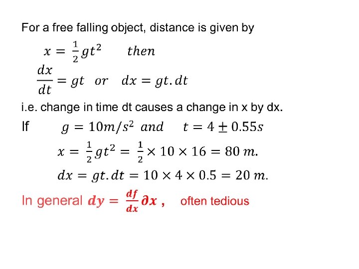
All measurements, how carefully done, involve errors These errors may be associated with technical difficulties Imperfection of measuring instrument, limitation of human eye and several other factors that can not be taken into account, like fluctuations in temperature, motion of air stream around the instrument

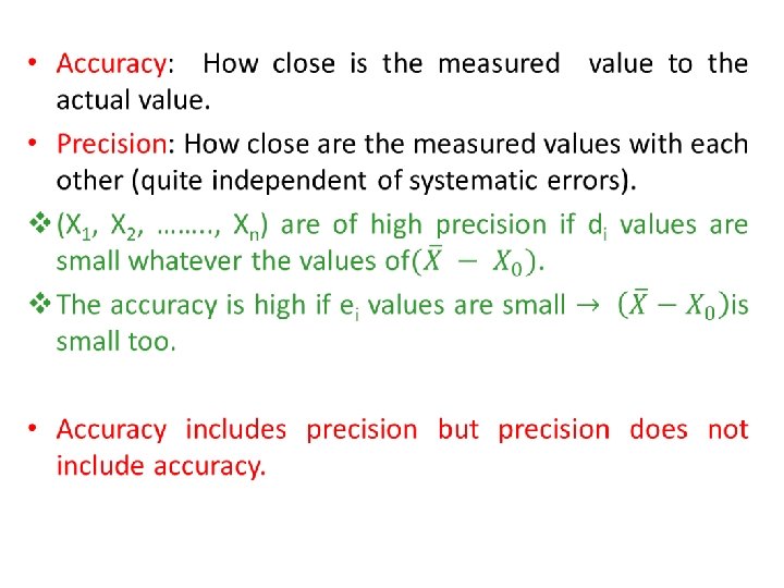
Accuracy How close a measured value is to the actual (true) value. Precision How close the measured values are to each other. Low Accuracy High Precision High Accuracy Low Precision High Accuracy High Precision

Accuracy signifies the degree of closeness between the measured value and true value of the quantity. Precision is the limit or resolution to which a quantity is measured. No matter how carefully we measure, we can never obtain a result more precise than the measuring device. The limit of precision of a measuring device is ±½ the smallest division of the device.

Significant Figures: Accuracy of measurements • While measuring a quantity, there is a limit to accuracy of measurement • This accuracy depends upon the number of digits upto which the value of a quantity is known. • It is, therefore, necessary to use appropriate number of digits to express the accuracy and reliability. • No purpose is served by writing additional digits. We can include only one more digit about which we are not sure. • The number of digits in a measurement about which we are reasonably sure plus the first uncertain digit are called significant figure.

Example: Length of an object is written as 2. 54 cm 3 significant figures 2. 5 is reliable. 3 rd figure, i. e. 4 is uncertain For a length of 638. 6 4 sig. fig. The last digit 6 is uncertain. Points to remember 1. Number of significant figures does not vary by varying the units selected 638. 6 cm = 6. 386 m 2. It is customary to write the decimal after the first digit 638. 6 cm = 6. 386 x 102 cm 0. 0438 kg = 4. 38 x 10 -2 kg

Rules for counting significant figures: 1. All non-zero digits are significant figures. If there is a decimal point, its position does not matter. 23. 73 has 4 sig. fig. 2. All zeros between two non-zero digits are significant figures and it does not matter where the decimal point occur. 2090. 03 has 6 sig. fig. 3. If there is no decimal point, zero at the end is meaning less and are not counted. 143000 has only 3 sig. fig. 4. If there is a decimal point, zeros at the end are significant. 36. 00 or 0. 3600 has 4 sig. fig. but Initial zeros after the decimal points are not significant, i. e. , zeros on the right of decimal and to the left of non-zero digits are not significant. 0. 0034 has only 2 sig. fig.

5. Zero on the left of decimal point for a number < 0 is never significant 6. A number with 3 significant figures (say) gives an accuracy of 1 part in 100 to 1000 A number with 6 significant figures (say) gives an accuracy of 1 part in 105 to 106. Rules of Rounding off the digits 9. 876 9. 88 Last digit > 5 9. 874 9. 87 Last digit < 5 If the last digit is 5, e. g. , 9. 775 9. 78 incremented by one if the last digit is odd. 9. 785 9. 78 no change in the last digit is even Rounding off should be such that the last digit should be even

Exercise: Two cesium clocks, if run for 100 years, free from disturbances may differ by only about 0. 02 s. What does this imply for the accuracy of the clock in measuring a time interval of 1 s. Time interval in 100 years = 100 x 365. 25 x 24 x 60 s Difference in the two clocks = 0. 02 s Measured time interval = 3155760000 ± 0. 02 = 3155760000. 02 or 3155759999. 98 Both these values have 12 sig. fig. The accuracy of the clock is 1 part in 1011 to 1012

= Alternative ΔT = 0. 02 s = 2 x 10 -2 s T = 100 years = 3. 15576 x 109 s ΔT/T = 6 x 10 -12 Accuracy ≈ 10 -11 to 10 -12 Rules for Arithmetic Operations with Significant Figures: Results from additions and subtractions are retained to the least decimal places that is present in the numbers being added/subtracted Sum or difference of the two or more numbers has significant figures only in those places where these are in the least precise amongst the given numbers 3. 123 + 40. 5 + 2. 0123 = 45. 7253

The answer should be only in three significant figures, i. e. 45. 7 (least accurate is 40. 5 and has only 3 sig. fig. ) Similarly 53. 312 – 53. 3 = 0. 012 But the answer should be 0. 0, as the least accurate is 53. 3 and has only one digit after decimal point Multiplication or Division of two numbers should have the sig. fig. that is present in the least precise of the given numbers, e. g. , 4. 08 x 16 = 65. 28 but the answer is 65, because the less precise number, 16 has only 2 sig. fig. Similarly, 6300/ 11. 97 = 526. 31578 but

The answer should be 530, because the less precise is 6300 which has 2 sig. fig Note: 3 rd digit is > 5 in 526. 31578 it is written as 530 Example: For a rectangular block, l = 4. 234 m, b = 1. 005 m, h = 2. 01 cm. Find the area and volume to correct sig. fig. Area = 4. 25517 m 2 = 4. 255 m 2 ( rounded off to 4 sig. fig. ) Volume = 0. 0855289 m 3 = 0. 0855 m 3 ( rounded off to 3 sig. fig. ) Example: Two masses, m 1 = 20. 15 g and m 2 = 20. 17 g Difference = 0. 02 g (one sig. fig) sig, fig. are lost in difference calculations

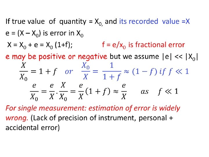
Errors in Measurements It is impossible to find a true value (in practice), while measuring a physical quantity Error: Difference in the measured and true value of a physical quantity. Degree of Accuracy depends on the instrument you are measuring with. But as a general rule: The degree of accuracy is half a unit each side of the unit of measure.

Examples: When the instrument measures in 1 unit then any value between 6½ and 7½ is measured as 7 units Thus, the value could be between 6½ and 7½ and is written as 7. 0 ± 0. 5 The error is ± 0. 5 When the instrument measures in 2 units then any value between 7 and 9 is measured as 8 units When the value lies between 7 and 9, it is written as 8± 1 The error is ± 1

Although Physics is exact science, physical instruments do not give the exact values of the quantities measured. All measurements in Physics/Science are inaccurate (generally) in some degree We often say that the true or actual value of a Physical quantity can not be found. We, however, assume that exact value exists and we concern to estimate the limits between which this value lies. The closer these limits, more accurate is the measurement.

Such errors follow no simple law and arise due to various causes. A single observer with the same apparatus will record different values of the same quantity. Errors are usually combination of accidental error and systematic errors Accidental Errors occur due to the observer and can be minimized by repeated observation. They are disordered. Systematic errors arise due to the observer or instrument and are usually more troublesome because repeated observations do not reveal them (usually) even when their nature of existence is known. It is difficult to determine and eliminate such errors

Assessment of possible errors in any measured quantity is of fundamental importance in science. Types of Errors • Accidental • Systematic • Random

Accidental errors estimated by certain statistical concepts. Systematic or personal errors assumed to be small and neglected. But sometimes it becomes rather a serious issue and special treatments are required for elimination Systematic errors of instrument

Systematic or Methodic Errors which tend to be in one direction, positive or negative and arise on account of Ø Short coming of measuring method Ø Imperfection of theory of physical phenomenon to which the quantity being measured is related to Ø Lack of accuracy of the formula used for calculations

e. g. Weighing a body on physical balance The systematic errors may be due to the fact that buoyant forces, acting on the body and weights, are not accounted Such errors may be reduced by Changing/improving the measuring method Applying corrections to the formula used

Instrumental Errors: Occur due to Ø imperfection of the design Ø inaccurate manufacturing of instrument e. g. , stop watch: running may change due to change in temperature or center of the dial may not coincide with the axis of rotation of its hands. It is not possible to eliminate such errors completely.

Random Errors: occur irregularly Arise due to the verity of the factors which can not be taken into account. These are not associated with any systematic cause or with definite law of action. e. g. , reading of a sensitive beam balance may be affected by the vibrations of the building or settling down the dust particles on the pan. Although such errors can not be completely eliminated, but can be reduced by repeated observations

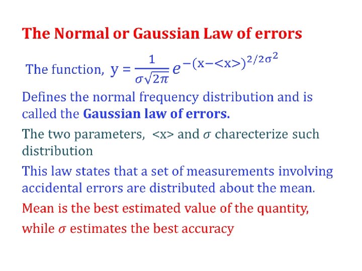
Random Errors are calculated on the basis of theory of probability by applying the Gaussian law of normal distribution R According to this law, probability of an error +ΔA in a measurement of a quantity A is the same as the probability of -ΔA in the very measurement Frequency -ΔA +ΔA Arithmetic mean of a large number of observations is likely to be closer to the true value

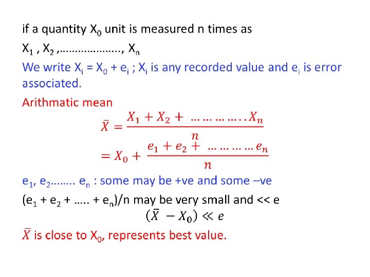
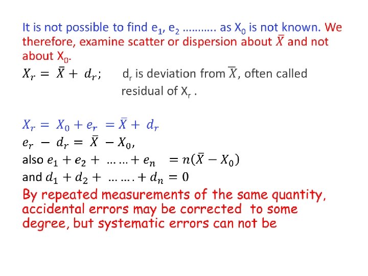
Absolute Errors Let A 1, A 2, …………. . An are the measured values of a quantity A in n attempts The arithmetic mean, Am = ΣAi/n Since the true value of the quantity is not known, Am may be considered as the true value. The magnitude of the deviation of any measurement from the arithmetic mean is called the absolute error of the measurement

Thus, the absolute errors are ΔA 1 = | Am – A 1| ΔA 1, ΔA 2 are magnitudes ΔA 2 = | Am – A 2| and are always taken as +ve Mean Absolute Error: Arithmetic mean of all the absolute errors Δ Am = Σ Δ Ai/n final absolute error The final results of the measurement is A = Am ± Δ Am

Any single measurement of quantity A is likely to be Am - ΔAm ≤ Am + ΔAm Relative or % of error = ΔAm/Am or (ΔAm/Am) x 100 %

Example: Diameter of a ball was measured five times whose absolute error is Δdinst = ± 0. 01 mm Observations are: d 1 = 5. 27 mm d 2 = 5. 30 mm d 3 = 5. 28 mm d 4 = 5. 33 mm d 5 = 5. 28 mm Find Mean value of diameter Mean absolute error Result of measurement Relative error and % of error Result with % of error Mean diameter dmean = (5. 27+5. 30+5. 28+5. 32+5. 28)/5 = 5. 29 mm

Absolute errors Δd 1 = dm – d 1 = 0. 02 mm Δd 2 = dm – d 2 = 0. 01 mm Δd 3 = dm – d 3 = 0. 01 mm Δd 4 = dm – d 4 = 0. 03 mm Δd 5 = dm – d 5 = 0. 02 mm Mean absolute error = (0. 02+0. 01+0. 03+0. 01)/5 Δdmean = 0. 02 mm Since Δdmean > Δdinst, result is dmean ± Δdmean = 5. 29± 0. 02 Relative error = Δdmean /dmean = 0. 02/5. 29= 0. 04 % of error = 4%

Example: A box is measured to the nearest 2 cm, and got 24 cm × 20 cm Measuring to the nearest 2 cm means the true value could be up to 1 cm smaller or larger. The three measurements are: l = 24 ± 1 cm b = 24 ± 1 cm h = 20 ± 1 cm The smallest possible Volume is: 23 cm × 19 cm = 10051 cm 3 The measured Volume is: 24 cm × 20 cm = 11520 cm 3 The largest possible Volume is: 25 cm × 21 cm = 13125 cm 3 Thus the measured value lies between 10051 and 13125

Absolute Error • From 10051 to 11520 = 1469 • From 11520 to 13125 = 1605 We pick the bigger one, i. e. , Absolute error = 1605 cm 3 Relative Error = 1605 cm 3 11520 cm 3 Percentage Error = 13. 9% = 0. 139. . .

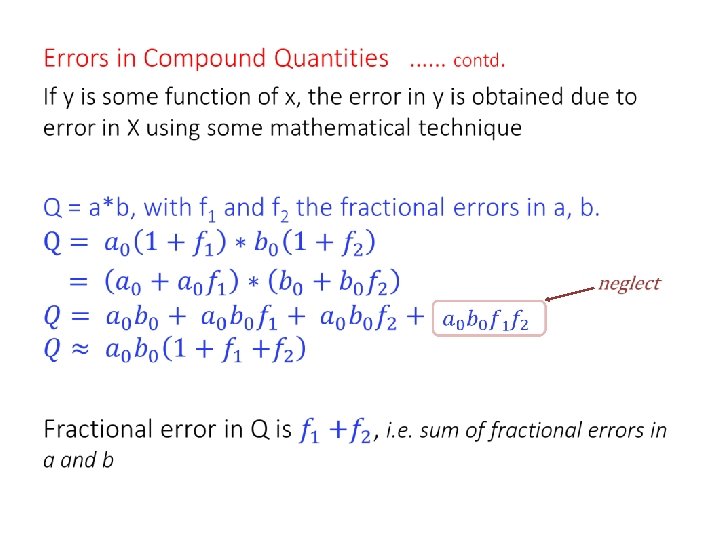
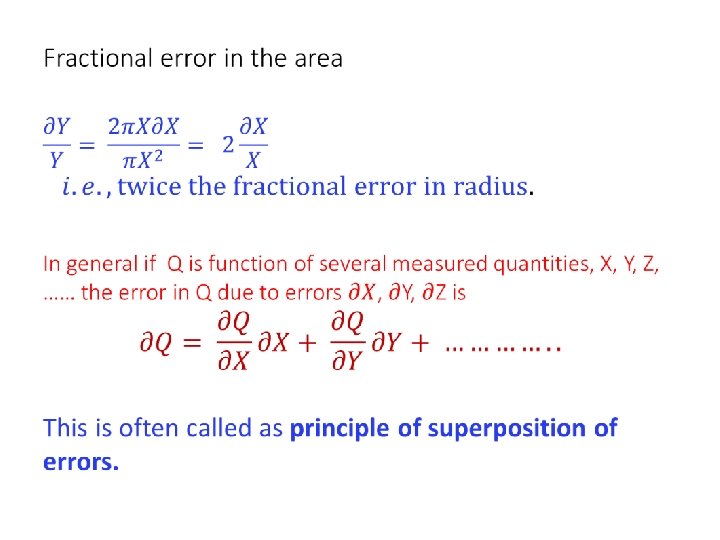
Combination/Propagation of Errors in Compound Quantities Errors in sum/difference A, B the two quantities with their errors as ΔA and ΔB respectively Measured value: (A ± ΔA) and (B ± ΔB) Let Z = A + B Z + ΔZ = (A ± ΔA) + (B ± ΔB) = (A + B) ± (ΔA + ΔB) ΔZ = ± (ΔA + ΔB) Maximum error in Z = (ΔA + ΔB) Similarly: for Z = A – B Z – ΔZ = (A-B) ± (ΔA + ΔB)

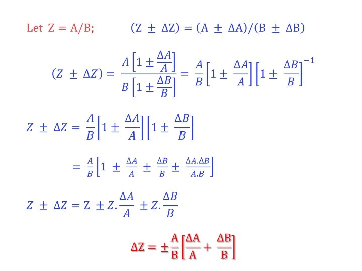
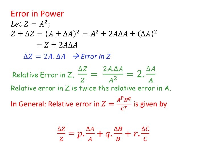
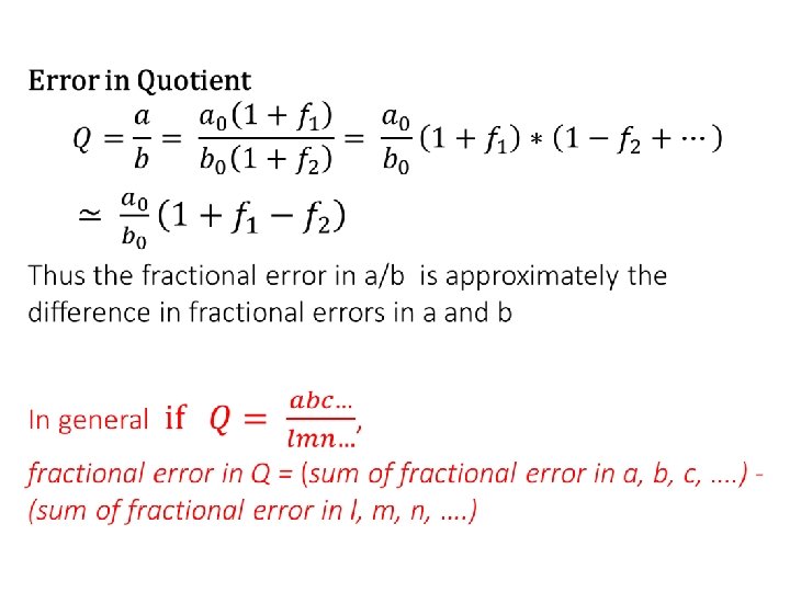
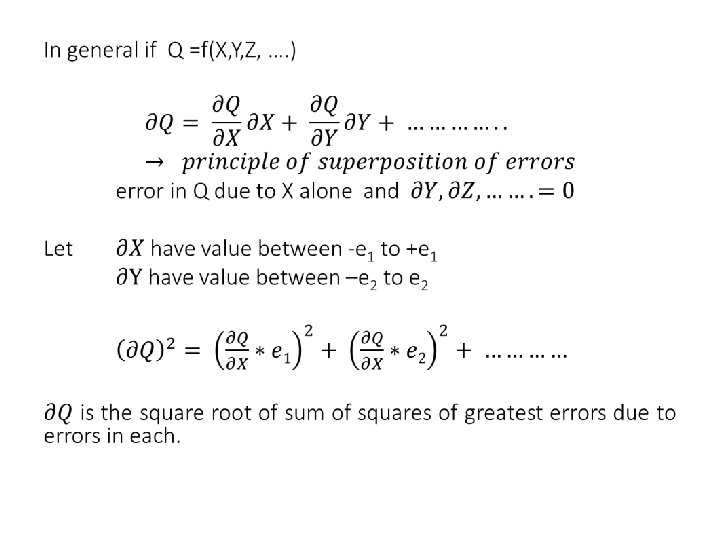
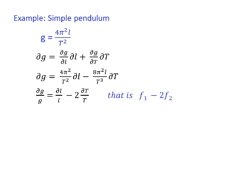
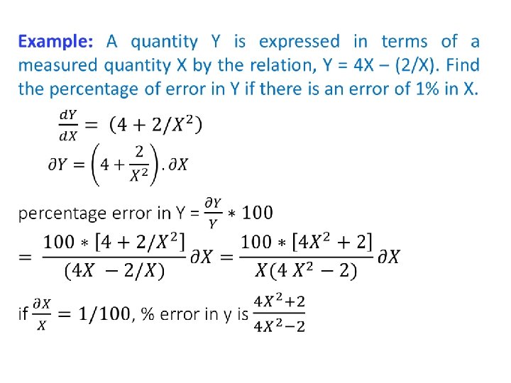
Errors in Product/Division

Some Statistical Ideas The experimental scientist does not regard statistics as an excuse for doing bad experiment. Frequency distributions: Numerical data on scientific measurements (and industrial and social statistics) are often represented graphically to aid their appreciation.

First step To arrange these in convenient order if they are large in numbers. This is often done by grouping them into classes according to their magnitude or according to suitable intervals of a variable on which they depend. The number of data in a particular class or group is usually called the frequency for that class

The following represents the frequency distribution of student’s marks (in %) in an exam Class Freq. 0 -9 2 50 -59 32 10 -19 5 60 -69 25 20 -29 6 70 -79 10 30 -39 14 80 -89 2 40 -49 22 90 -99 2 Width of class is the difference between the 1 st numbers of two consecutive classes, i. e. 10 here From the table one can appreciate the distribution of marks But Graphically.

Frequency Distribution Polygon Bar Graph

Frequency Distribution Histogram

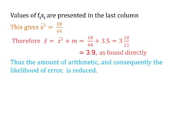
Histogram: A series of rectangles are constructed of width equal to class width and area equal to frequency of the corresponding class. The areas are 2, 5, 6, 14, . . . units. Total area of histogram = 120 units = total no. of students. The heights of rectangles are proportional to freq. when classes are of equal width. In this case, the mean height of rectangles = mean frequency

• xi fi fixi 0. 5 1 0. 5 -3 -3 1. 5 5 7. 5 -2 -10 2. 5 7 17. 5 -1 -77 3. 5 9 31. 5 0 0 4. 5 10 45. 0 1 10 5. 5 8 44. 0 2 16 6. 5 4 26. 0 3 12 SUM 44 172. 0 18

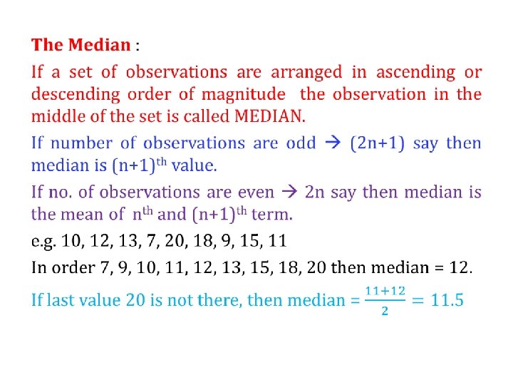
To find the Median, place the numbers you are given in order and find the middle number. To find the median of {13, 23, 11, 16, 15, 10, 26}. We put them in order: {10, 11, 13, 15, 16, 23, 26} The middle number is 15, so the median is 15. (If there are two middle numbers, average of the two is taken. )

MODE: The number which appears most often in a set of numbers. in {6, 3, 9, 6, 6, 5, 9, 3} the Mode is 6 (it occurs most often). Mode corresponds to maximum frequency. The histogram tends to be more and more close to the frequency curve as the number of observations increases.

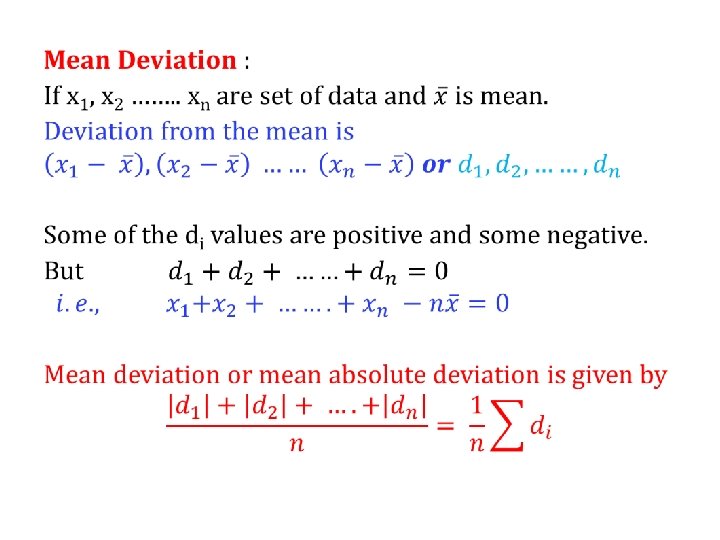
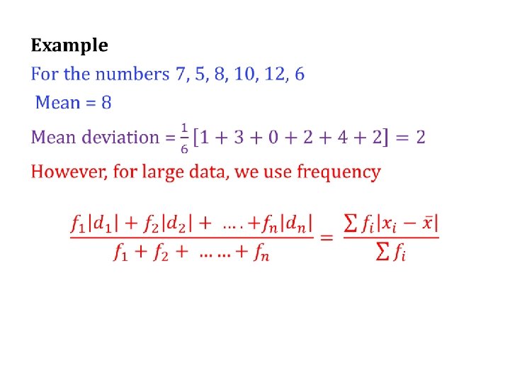
The Mean Deviation The mean of the distances of each value from their mean. Three steps to find the mean deviation • Find the mean of all values • Find the distance of each value from that mean (subtract the mean from each value, ignore minus signs) • Then find the mean of those distances

Mean Deviation of 3, 6, 6, 7, 8, 11, 15, 16 Mean = (3+6+6+7+8+11+15+16)/8 = 72/8 = 9 distance of each value from that mean is evaluated as Mean deviation = (6+3+3+2+1+2+6+7)/8 = 30/8 = 3. 75 It tells how far, on average, all values are from the middle Value 3 6 6 7 8 11 15 16 Distance from 9 6 3 3 2 1 2 6 7

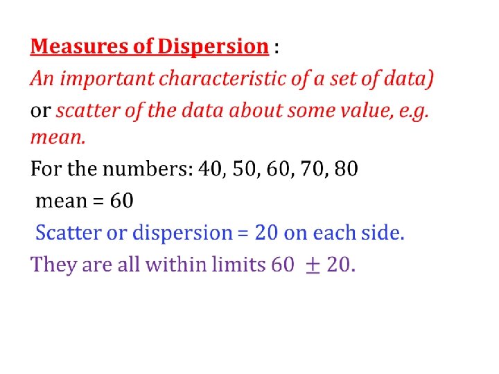
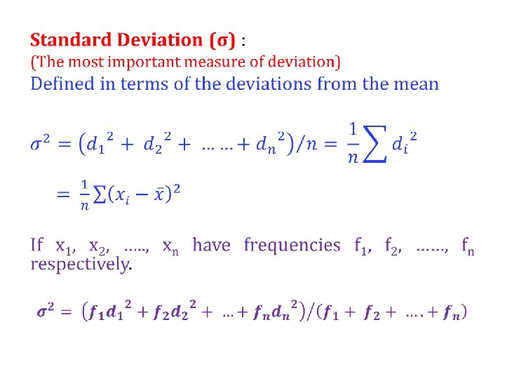
Various parameters are used to measure dispersion. 1. Range 2. Mean deviation 3. Standard deviation Range of freq. distribution = max value – min value of variable. It is a simple measure of dispersion but has limitations due to simplicity.

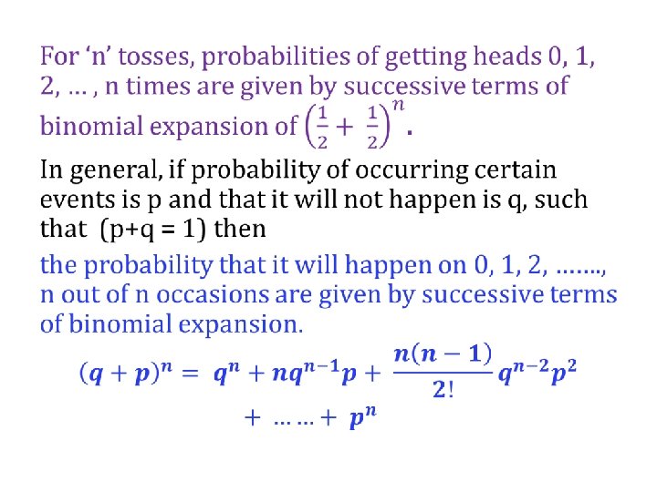
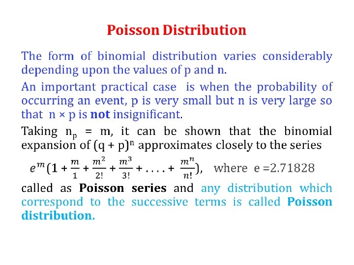
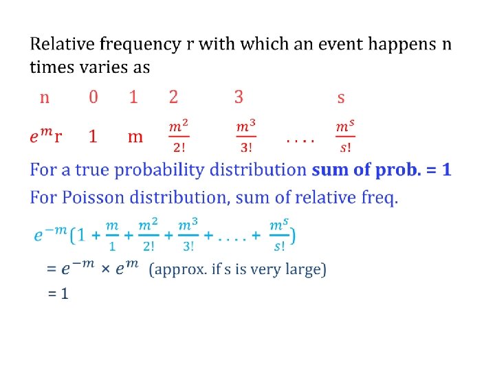
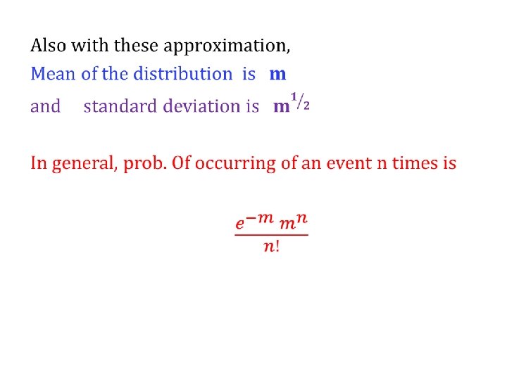
Frequency Distributions (Three important Types) 1. Binomial 2. Poisson 3. Normal Most of the distribution, based on scientific observations or industrial and social statistics approach closely to on or the other of these three important distributions. These distributions can be derived and expressed mathematically using theory of prob.

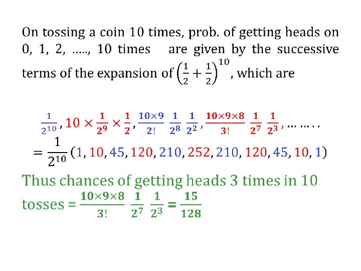
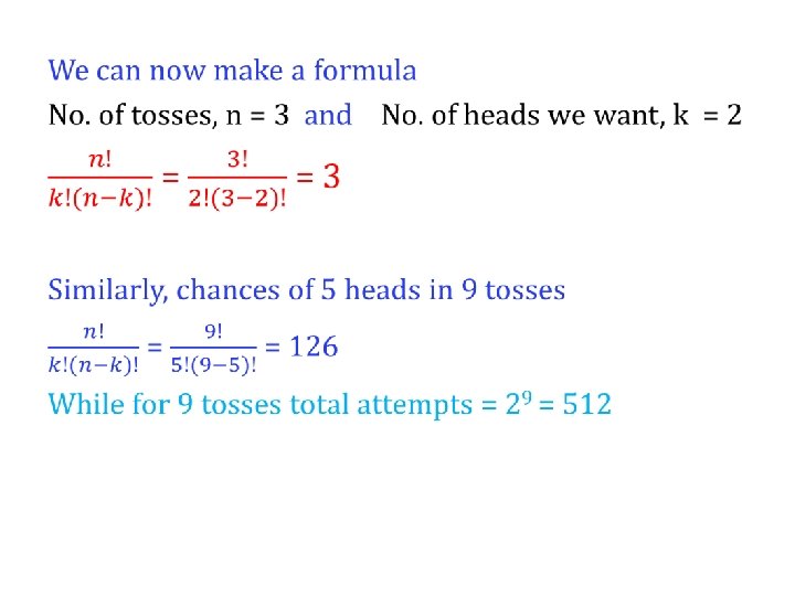
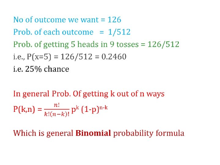
The Binomial distribution: On tossing a coin we have two probabilities Heads or tails i. e. , chances of getting heads or tails is 50% For ‘n’ number of tosses (n is large) No. of times we get heads ≈ n/2. For small n, chances of deviation from 50% are large Tossing a coin 10 times For another 10 tosses we may get heads 3 times we may get heads 6 times Question: On tossing ‘n’ times what is the chance of getting heads ‘m’ times? 0≤ m ≤ n.

If we toss a coin 3 times, we can get HHH HHT HTH HTT THH THT TTH TTT Each outcome is equally likely, and there are 8 of them. So each has a probability of 1/8 So the probability of “two Heads" in “three tosses” is: Total No. of Attempts 23 = 8 No. of outcome Prob. of each we want outcome 3 X 1/8 = 3/8

Thus we have • • P(3 -heads) = P(HHH) = 1/8 P(2 -Heads) = P(HHT) + P(HTH) + P(THH) = 1/8 + 1/8 = 3/8 P(1 -Head) = P(HTT) + P(THT) + P(TTH) = 1/8 + 1/8 = 3/8 P(Zero Heads) = P(TTT) = 1/8 We can write this in terms of a Random Variable, X • P(X = 3) = 1/8 • P(X = 2) = 3/8 • P(X = 1) = 3/8 • P(X = 0) = 1/8

m=3 m=5 m = 10

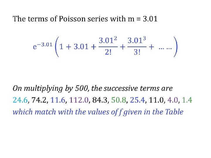
• n 0 1 2 3 4 5 6 7 8 9 SUM f 24 77 110 112 84 50 24 12 5 2 500 n×f 0 77 220 336 250 144 84 40 18 1505 24. 6 74. 2 84. 3 50. 8 25. 4 11. 0 4 11. 6 112. 0

Using an assumed mean = 3, d = n-3, we may tabulate n d=n-3 fd fd 2 0 -3 -72 216 1 -2 -154 308 2 -1 -110 3 0 0 0 4 1 84 84 5 2 100 200 6 3 72 216 7 4 48 192 8 5 25 125 9 6 12 72 sum 5 1523

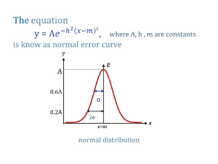
Normal Distribution • Discovered in 1733 by de Moivre as an approximation to the binomial distribution when the number of trails is large • Also obtained by Laplace and Gauss later • Importance lies in the Central Limit Theorem, which states that the sum of a large number of independent random variables (binomial, Poisson, etc. ) will approximate a normal distribution

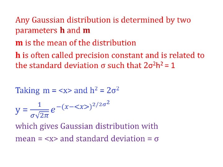
Gaussian distribution for the same mean and different σ

Example From a sample of fish in a pond it is found that the mean length of these fish, m is 30 cm while 2 = 4 cm We assume that the length is normal random variable If we catch one of these fish the what is the probability that • it will be at least 31 cm. long? • it will be no more than 32 cm. long? • its length will be between 26 and 29 cm?

Prob. that it will be 31 cm long

P Prob. that it will be less than 32 cm

Prob. that it length will be between 28 and 30 cm

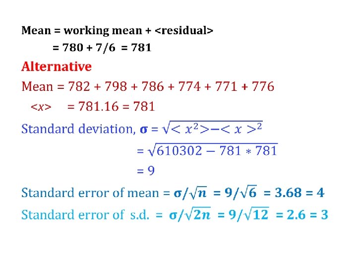
Example: Values of distances covered by a tourist on a vehicle are listed ( in km/day). Find the mean distance and its standard error 782 798 786 774 771 776 sum Working mean = 780 Residual d 2 18 6 d 2 4 324 36 -6 -9 -4 7 36 81 16 497

Standard Errors of Compound Quantities If a number of measured quantities have means m 1, m 2, m 3, . . mn with standard errors α 1, α 2, α 3, . . , αn respectively then the standard error of Quantity Error The sum m 1+ m 2 The difference m 1 - m 2 The multiple km 1 The product m 1 m 2 m 3 Power

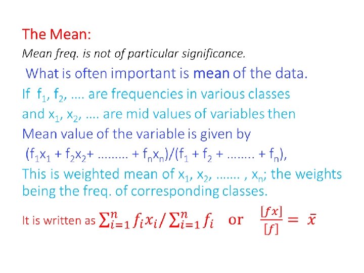
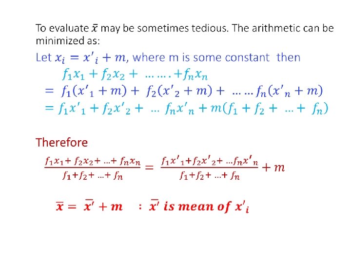
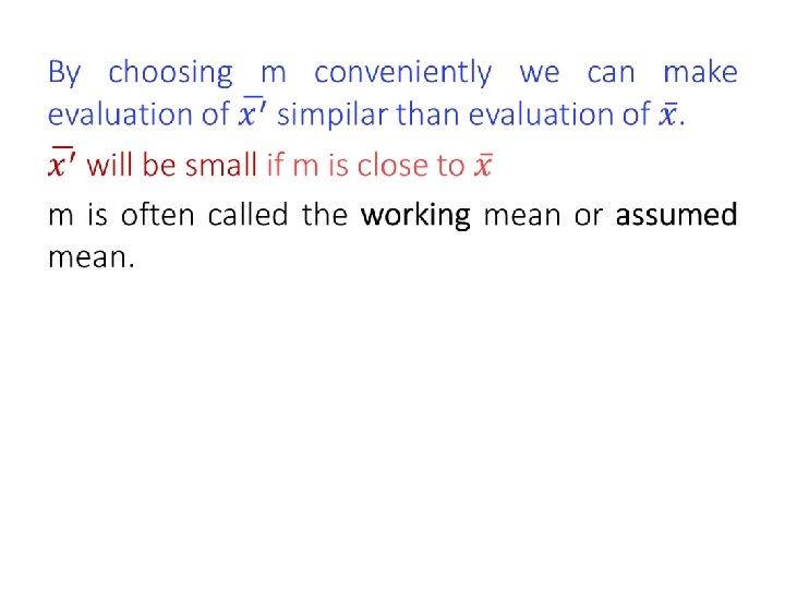
Weighted mean A mean where some values contribute more than others. When we do a simple mean (or average), we give equal weight to each number. mean = (1 + 2 + 3 + 4)/4 = 2. 5 Each of the four numbers has a weight of ¼ Mean = ¼× 1 + ¼× 2 + ¼× 3 + ¼× 4 = 0. 25 + 0. 75 +1. 0 = 2. 5

If weight of 3 is changed to 0. 7, the other three numbers have still equal weights of 0. 1 each so that total weight is 1 Mean = 0. 1 × 1 + 0. 1 × 2 + 0. 7 × 3+ 0. 1 × 4 = 2. 8 This weighted mean is now a little higher ("pulled" there by the weight of 3). When some values get more weight than others the central point (the mean) can change:

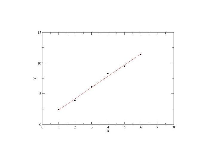
• x y ycal d d 2 1. 0 2. 4 2. 3 0. 1 0. 01 2. 0 3. 9 4. 1 0. 2 0. 04 3. 0 6. 1 5. 9 0. 2 0. 04 4. 0 8. 3 7. 7 0. 6 0. 36 5. 0 9. 5 0. 00 6. 0 11. 4 11. 3 0. 1 0. 01

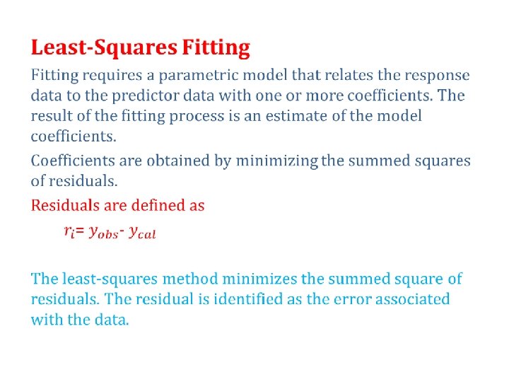
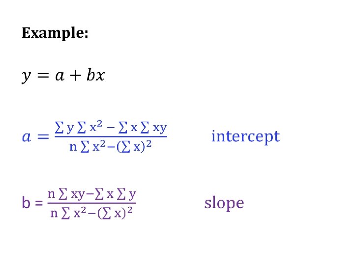
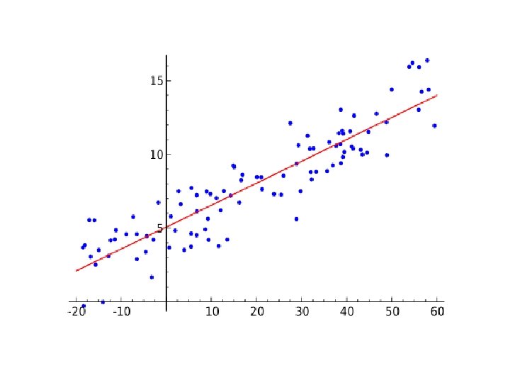
Fitting • To find a functional form that describes data within errors • Why fit data? • Extract physical parameters from data • Test validity of data or model • Interpolate/extrapolate data

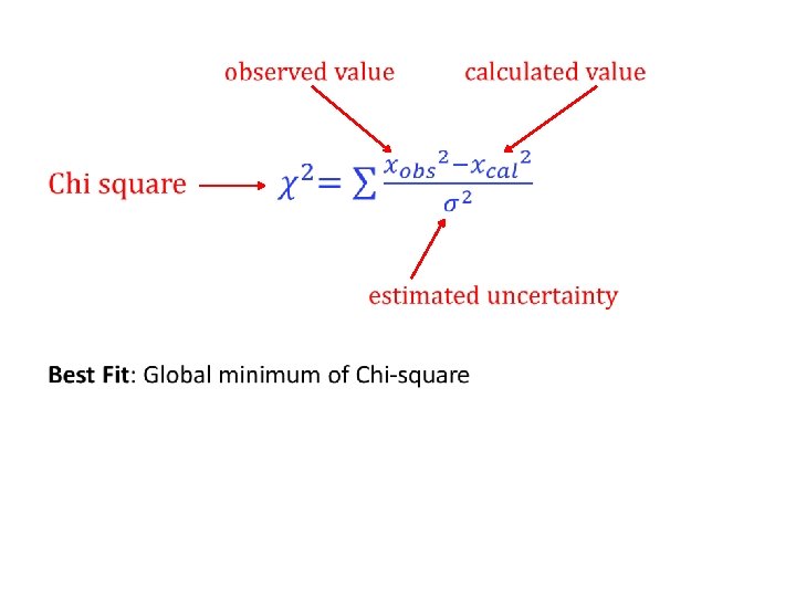
Goodness of fit • Data are expected to fluctuate by ~ error • Chi-square per Degree of Freedom (Do. F) should be ~ 1 • Do. F: Number of data points - number of fitted parameters • Chi-square allows to test if model/fitted function is compatible with data

How to fit data? Vary parameters of function until you find a global maximum of goodness-of-fit criterion Goodness-of-fit • chi-square (most common) • likelihood • (Kolmogorov-Smirnov test)

X Y± Error X 2 X. Y Ycal d 2 χ2 1 5. 1 ± 0. 6 1 5. 1 4. 83 0. 072 0. 202 2 10. 2 ± 0. 9 4 20. 4 9. 96 0. 057 0. 071 3 14. 7 ± 1. 4 9 44. 1 15. 09 0. 152 0. 077 4 19. 5 ± 1. 8 16 78. 0 20. 22 0. 518 0. 160 5 25. 9 ± 2. 2 25 129. 5 25. 35 0. 302 0. 062 6 30. 7 ± 3. 3 36 184. 2 30. 48 0. 004 ΣX=21 , ΣY=106. 1 , ΣX 2=91 , Σd 2=1. 149 , Σ χ2=0. 576 ΣX. Y=461. 3

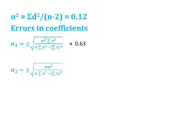
= - 0. 3 = 5. 13 = 0. 287

= ± 0. 460 = ± 0. 118 Which gives : Ycal = -0. 3 ± 0. 460 + (5. 13± 0. 118)X And = 0. 144

Chi-square distribution Even if the error estimate is correct and the model is correct • Chi-square will fluctuate from chi 2/Do. F < 1 to chi 2/Do. F > 1 • The shape of the chi 2 -distribution depends only on the number of degrees of freedom • Probability that data and model agree can be calculated Chi-square probability Percentage of all measurements that have a worse chi-square than expected

Books 1. Ideas about Errors by J. Topping 2. A Practical Guide to Data analysis for Physical Science Students by Louis Lyons Few figures taken from the net

Thank you