Statistics Statistical Tests Assumptions Conclusions Kinds of degrees

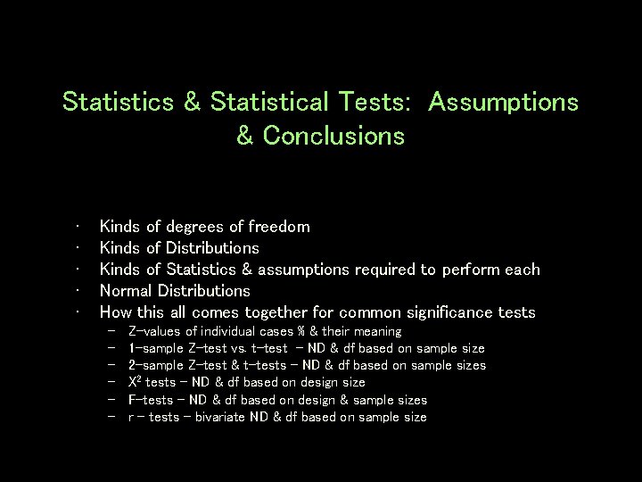
Statistics & Statistical Tests: Assumptions & Conclusions • • • Kinds of degrees of freedom Kinds of Distributions Kinds of Statistics & assumptions required to perform each Normal Distributions How this all comes together for common significance tests – – – Z-values of individual cases % & their meaning 1 -sample Z-test vs. t-test – ND & df based on sample size 2 -sample Z-test & t-tests – ND & df based on sample sizes X 2 tests – ND & df based on design size F-tests – ND & df based on design & sample sizes r – tests – bivariate ND & df based on sample size

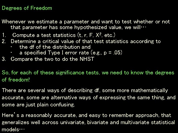
Degrees of Freedom Whenever we estimate a parameter and want to test whether or not that parameter has some hypothesized value, we will… 1. Compute a test statistics (t, r, F, X 2, etc. ) 2. Determine a critical value of that test statistics according to • the df of the distribution and • a specified Type I error rate (e. g. , p =. 05) 3. Compare the two to do the NHST So, for each of these significance tests, we need to know the degrees of freedom! There are several ways of describing df, some more mathematically accurate, some are alternative ways of expressing the same thing, and some are just plain confusing. Here’s a reasonably accurate, and easy to remember approach, that generalizes well across univariate, bivariate and multivariate statistical models…

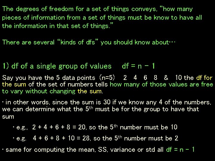
The degrees of freedom for a set of things conveys, “how many pieces of information from a set of things must be know to have all the information in that set of things. ” There are several “kinds of dfs” you should know about… 1) df of a single group of values df = n - 1 Say you have the 5 data points (n=5) 2 4 6 8 & 10 the df for the sum of the set of numbers tells how many of those values are free to vary without changing the sum. • in other words, since the sum is 30 if we know any 4 of the numbers, we can determine what the 5 th must be for the group to have that sum • e. g. , 2 + 4 + 6 + 8 = 20, so the 5 th number must be 10 • e. g. 4 + 6 + 8 + 10 = 28, so the 5 th number must be 2 • same for computing the mean, SS, variance or std all df = n – 1

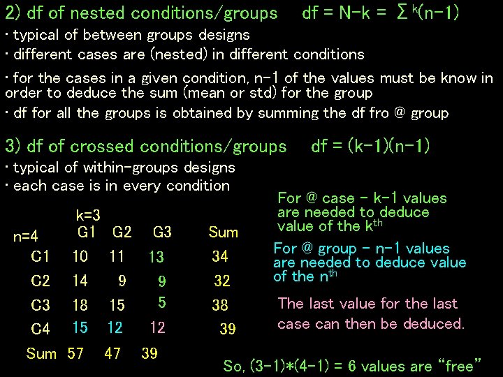
2) df of nested conditions/groups df = N-k = Σk(n-1) • typical of between groups designs • different cases are (nested) in different conditions • for the cases in a given condition, n-1 of the values must be know in order to deduce the sum (mean or std) for the group • df for all the groups is obtained by summing the df fro @ group 3) df of crossed conditions/groups • typical of within-groups designs • each case is in every condition k=3 G 1 10 14 18 15 n=4 C 1 C 2 C 3 C 4 Sum 57 G 2 G 3 11 13 9 9 5 15 12 12 47 39 Sum 34 32 38 39 df = (k-1)(n-1) For @ case – k-1 values are needed to deduce value of the kth For @ group – n-1 values are needed to deduce value of the nth The last value for the last case can then be deduced. So, (3 -1)*(4 -1) = 6 values are “free”

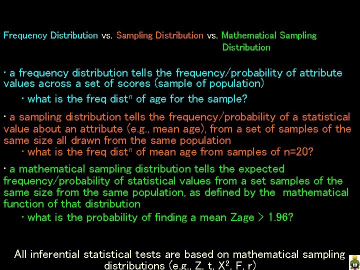
Frequency Distribution vs. Sampling Distribution vs. Mathematical Sampling Distribution • a frequency distribution tells the frequency/probability of attribute values across a set of scores (sample of population) • what is the freq distn of age for the sample? • a sampling distribution tells the frequency/probability of a statistical value about an attribute (e. g. , mean age), from a set of samples of the same size all drawn from the same population • what is the freq distn of mean age from samples of n=20? • a mathematical sampling distribution tells the expected frequency/probability of statistical values from a set samples of the same size from the same population, as defined by the mathematical function of that distribution • what is the probability of finding a mean Zage > 1. 96? All inferential statistical tests are based on mathematical sampling distributions (e. g. , Z, t, X 2, F, r)

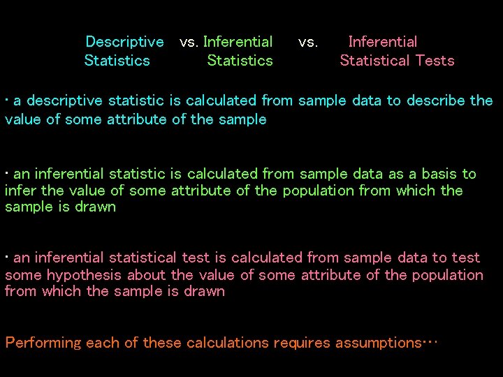
Descriptive vs. Inferential Statistics vs. Inferential Statistical Tests • a descriptive statistic is calculated from sample data to describe the value of some attribute of the sample • an inferential statistic is calculated from sample data as a basis to infer the value of some attribute of the population from which the sample is drawn • an inferential statistical test is calculated from sample data to test some hypothesis about the value of some attribute of the population from which the sample is drawn Performing each of these calculations requires assumptions…

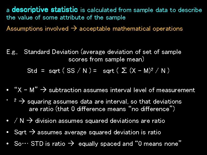
a descriptive statistic is calculated from sample data to describe the value of some attribute of the sample Assumptions involved acceptable mathematical operations E. g. , Standard Deviation (average deviation of set of sample scores from sample mean) Std = sqrt ( SS / N ) = sqrt ( ∑ (X – M)2 / N ) • “X – M” subtraction assumes interval level of measurement • 2 squaring assumes data are interval, so that deviations are ratio (that 0 difference means “no difference”) • / N division assumes squared deviations are ratio • Sqrt assumes average squared deviation is ratio • So… STD is ratio equally spaced and “ 0 means none”

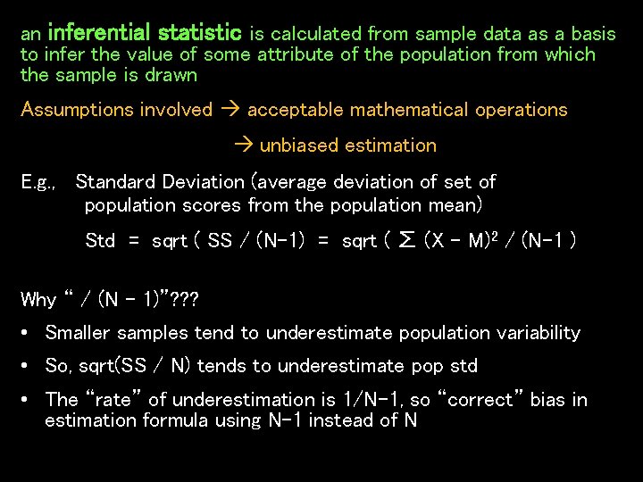
an inferential statistic is calculated from sample data as a basis to infer the value of some attribute of the population from which the sample is drawn Assumptions involved acceptable mathematical operations unbiased estimation E. g. , Standard Deviation (average deviation of set of population scores from the population mean) Std = sqrt ( SS / (N-1) = sqrt ( ∑ (X – M)2 / (N-1 ) Why “ / (N – 1)”? ? ? • Smaller samples tend to underestimate population variability • So, sqrt(SS / N) tends to underestimate pop std • The “rate” of underestimation is 1/N-1, so “correct” bias in estimation formula using N-1 instead of N

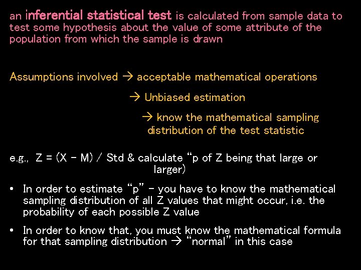
an inferential statistical test is calculated from sample data to test some hypothesis about the value of some attribute of the population from which the sample is drawn Assumptions involved acceptable mathematical operations Unbiased estimation know the mathematical sampling distribution of the test statistic e. g. , Z = (X – M) / Std & calculate “p of Z being that large or larger) • In order to estimate “p” – you have to know the mathematical sampling distribution of all Z values that might occur, i. e. the probability of each possible Z value • In order to know that, you must know the mathematical formula for that sampling distribution “normal” in this case

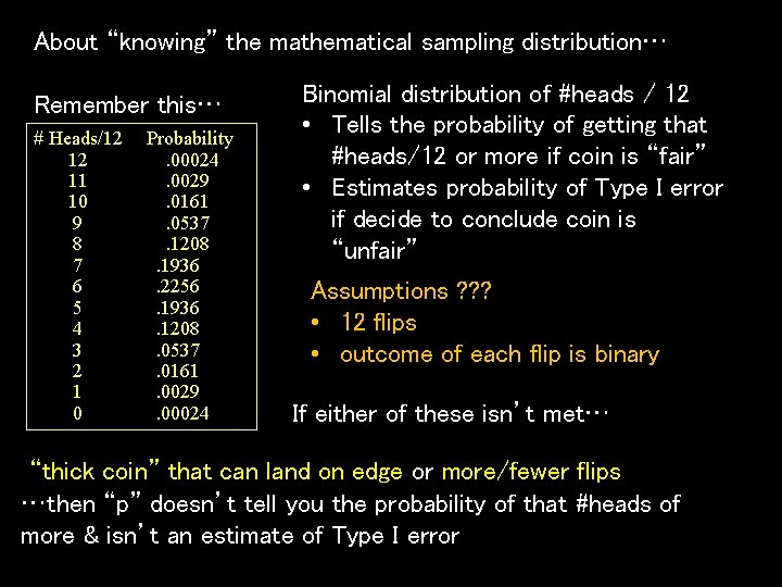
About “knowing” the mathematical sampling distribution… Remember this… # Heads/12 12 11 10 9 8 7 6 5 4 3 2 1 0 Probability. 00024. 0029. 0161. 0537. 1208. 1936. 2256. 1936. 1208. 0537. 0161. 0029. 00024 Binomial distribution of #heads / 12 • Tells the probability of getting that #heads/12 or more if coin is “fair” • Estimates probability of Type I error if decide to conclude coin is “unfair” Assumptions ? ? ? • 12 flips • outcome of each flip is binary If either of these isn’t met… “thick coin” that can land on edge or more/fewer flips …then “p” doesn’t tell you the probability of that #heads of more & isn’t an estimate of Type I error

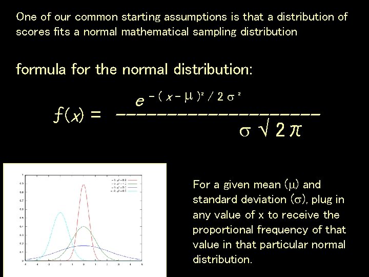
One of our common starting assumptions is that a distribution of scores fits a normal mathematical sampling distribution formula for the normal distribution: e - ( x - )² / 2 ² ƒ(x) = ---------- 2π For a given mean ( ) and standard deviation ( ), plug in any value of x to receive the proportional frequency of that value in that particular normal distribution.

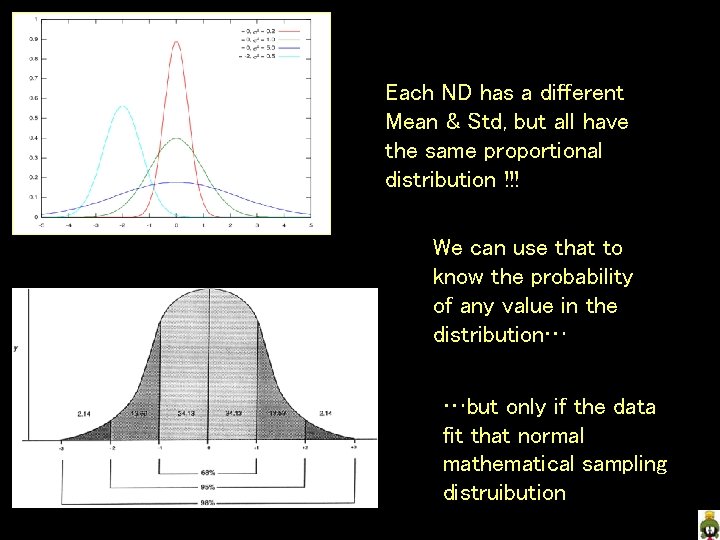
Each ND has a different Mean & Std, but all have the same proportional distribution !!! We can use that to know the probability of any value in the distribution… …but only if the data fit that normal mathematical sampling distruibution

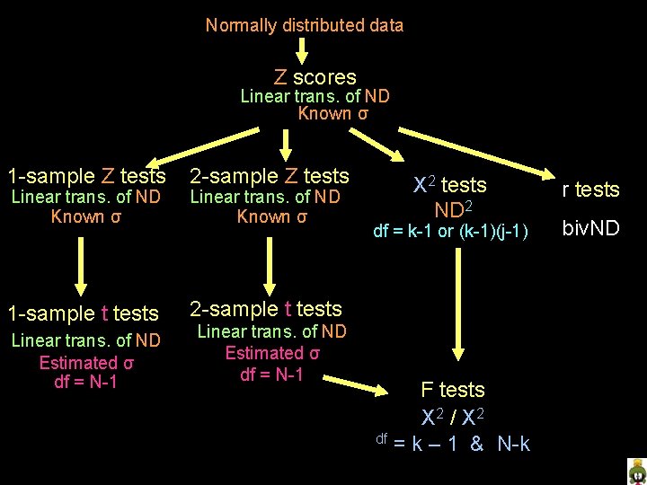
Normally distributed data Z scores Linear trans. of ND Known σ 1 -sample Z tests Linear trans. of ND Known σ 1 -sample t tests Linear trans. of ND Estimated σ df = N-1 2 -sample Z tests Linear trans. of ND Known σ X 2 tests ND 2 df = k-1 or (k-1)(j-1) 2 -sample t tests Linear trans. of ND Estimated σ df = N-1 F tests X 2 / X 2 df = k – 1 & N-k r tests biv. ND

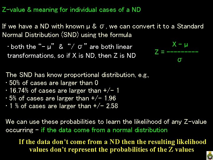
Z-value & meaning for individual cases of a ND If we have a ND with known µ & σ, we can convert it to a Standard Normal Distribution (SND) using the formula X-µ • both the “- µ” & “/ σ” are both linear Z = ----transformations, so if X is ND, then Z is ND σ The SND has know proportional distribution, e. g. , • 50% of cases are larger than 0 • 16. 74% of cases are larger than +/- 1 • 5% of cases are larger than +/- 1. 96 • 1 % of cases are larger than +/- 2. 58 We can use these probabilities to learn the likelihood of any Z-value occurring – if the data come from a normal distribution If the data don’t come from a ND then the resulting likelihood values don’t represent the probabilities of the Z values

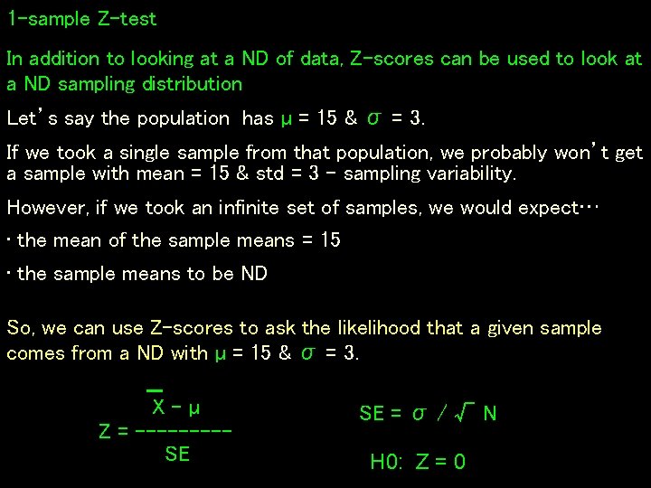
1 -sample Z-test In addition to looking at a ND of data, Z-scores can be used to look at a ND sampling distribution Let’s say the population has µ = 15 & σ = 3. If we took a single sample from that population, we probably won’t get a sample with mean = 15 & std = 3 – sampling variability. However, if we took an infinite set of samples, we would expect… • the mean of the sample means = 15 • the sample means to be ND So, we can use Z-scores to ask the likelihood that a given sample comes from a ND with µ = 15 & σ = 3. X-µ Z = ----SE SE = σ / √ N H 0: Z = 0

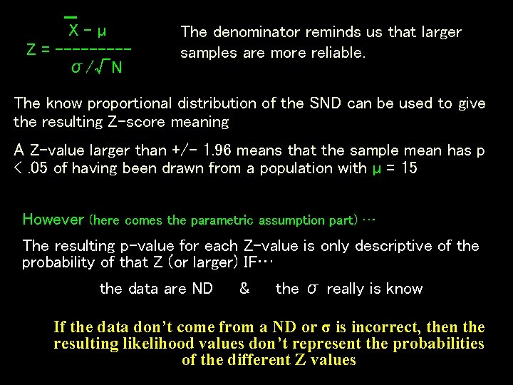
X-µ Z = ----σ/√N The denominator reminds us that larger samples are more reliable. The know proportional distribution of the SND can be used to give the resulting Z-score meaning A Z-value larger than +/- 1. 96 means that the sample mean has p <. 05 of having been drawn from a population with µ = 15 However (here comes the parametric assumption part) … The resulting p-value for each Z-value is only descriptive of the probability of that Z (or larger) IF… the data are ND & the σ really is know If the data don’t come from a ND or σ is incorrect, then the resulting likelihood values don’t represent the probabilities of the different Z values

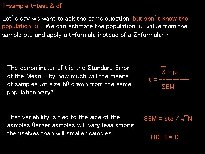
1 -sample t-test & df Let’s say we want to ask the same question, but don’t know the population σ. We can estimate the population σ value from the sample std and apply a t-formula instead of a Z-formula… The denominator of t is the Standard Error of the Mean – by how much will the means of samples (of size N) drawn from the same population vary? That variability is tied to the size of the samples (larger samples will vary less among themselves than will smaller samples) X-µ t = ----SEM = std / √N H 0: t = 0

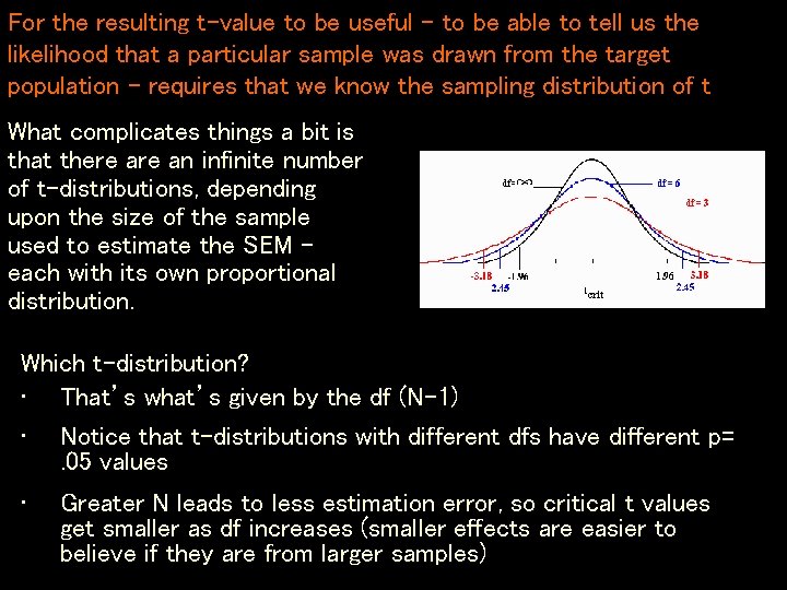
For the resulting t-value to be useful – to be able to tell us the likelihood that a particular sample was drawn from the target population – requires that we know the sampling distribution of t What complicates things a bit is that there an infinite number of t-distributions, depending upon the size of the sample used to estimate the SEM – each with its own proportional distribution. Which t-distribution? • That’s what’s given by the df (N-1) • Notice that t-distributions with different dfs have different p=. 05 values • Greater N leads to less estimation error, so critical t values get smaller as df increases (smaller effects are easier to believe if they are from larger samples)

However (here comes the parametric assumption part) … The resulting p-value for each t-value is only descriptive of the probability of that t (or larger) IF… • the data from which the mean and SEM are calculated are really ND • if the data aren’t ND, then … • the value computed from the formula isn’t distributed as t with that df and … • the p-value doesn’t mean what we think it means So, ND assumptions have the roll we said before… If the data aren’t ND, then the resulting summary statistic from the inferential statistical test isn’t distributed as expected (i. e. , as t with a specified df = n-1), and the resulting p-value doesn’t tell us the probability of finding that large of a t (or larger) if H 0: is true!

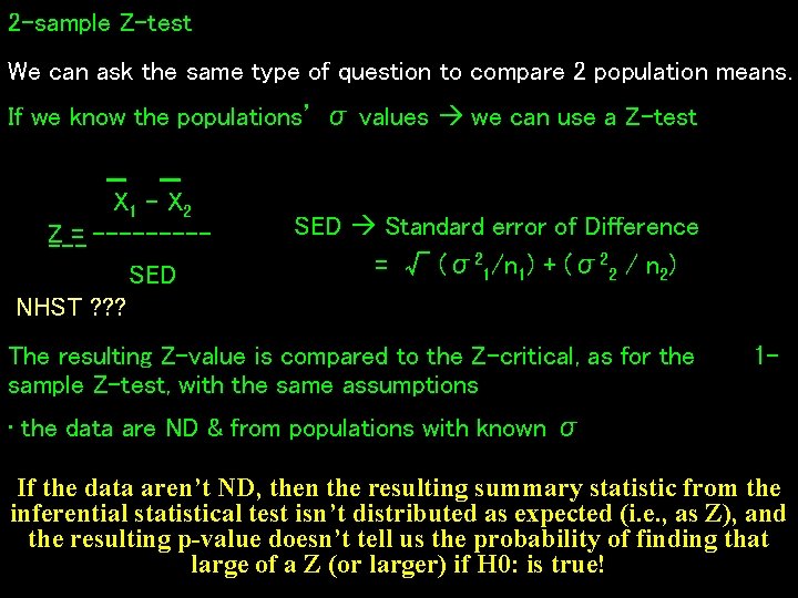
2 -sample Z-test We can ask the same type of question to compare 2 population means. If we know the populations’ σ values we can use a Z-test X 1 – X 2 Z = -----SED Standard error of Difference = √ (σ21/n 1) + (σ22 / n 2) NHST ? ? ? The resulting Z-value is compared to the Z-critical, as for the sample Z-test, with the same assumptions 1 - • the data are ND & from populations with known σ If the data aren’t ND, then the resulting summary statistic from the inferential statistical test isn’t distributed as expected (i. e. , as Z), and the resulting p-value doesn’t tell us the probability of finding that large of a Z (or larger) if H 0: is true!

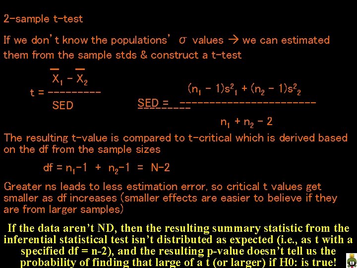
2 -sample t-test If we don’t know the populations’ σ values we can estimated them from the sample stds & construct a t-test X 1 – X 2 t = ----SED (n 1 – 1)s 21 + (n 2 – 1)s 22 SED = ---------------- n 1 + n 2 - 2 The resulting t-value is compared to t-critical which is derived based on the df from the sample sizes df = n 1 -1 + n 2 -1 = N-2 Greater ns leads to less estimation error, so critical t values get smaller as df increases (smaller effects are easier to believe if they are from larger samples) If the data aren’t ND, then the resulting summary statistic from the inferential statistical test isn’t distributed as expected (i. e. , as t with a specified df = n-2), and the resulting p-value doesn’t tell us the probability of finding that large of a t (or larger) if H 0: is true!

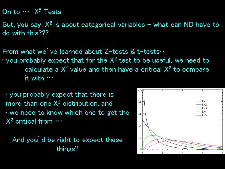
On to … X 2 Tests But, you say, X 2 is about categorical variables – what can ND have to do with this? ? ? From what we’ve learned about Z-tests & t-tests… • you probably expect that for the X 2 test to be useful, we need to calculate a X 2 value and then have a critical X 2 to compare it with … • you probably expect that there is more than one X 2 distribution, and • we need to know which one to get the X 2 critical from … And you’d be right to expect these things!!

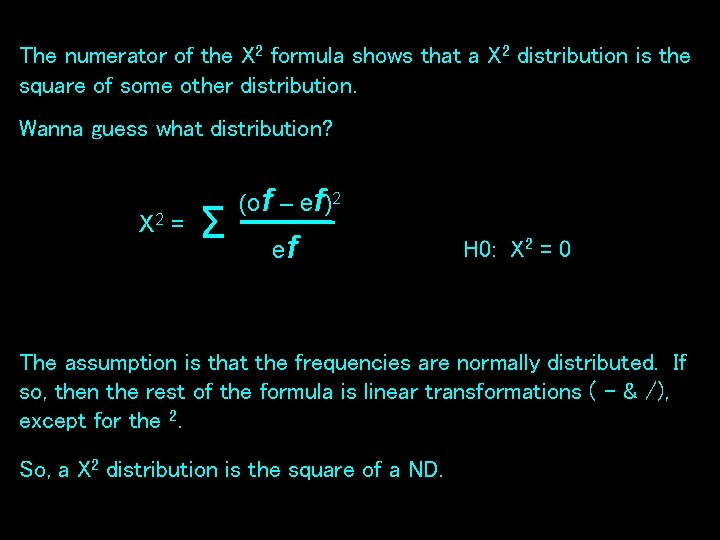
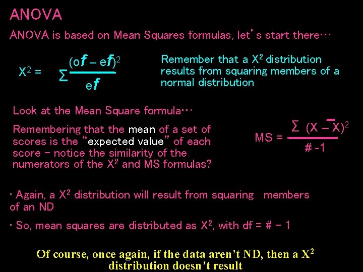
The numerator of the X 2 formula shows that a X 2 distribution is the square of some other distribution. Wanna guess what distribution? X 2 = Σ (of – ef)2 ef H 0: X 2 = 0 The assumption is that the frequencies are normally distributed. If so, then the rest of the formula is linear transformations ( - & /), except for the 2. So, a X 2 distribution is the square of a ND.

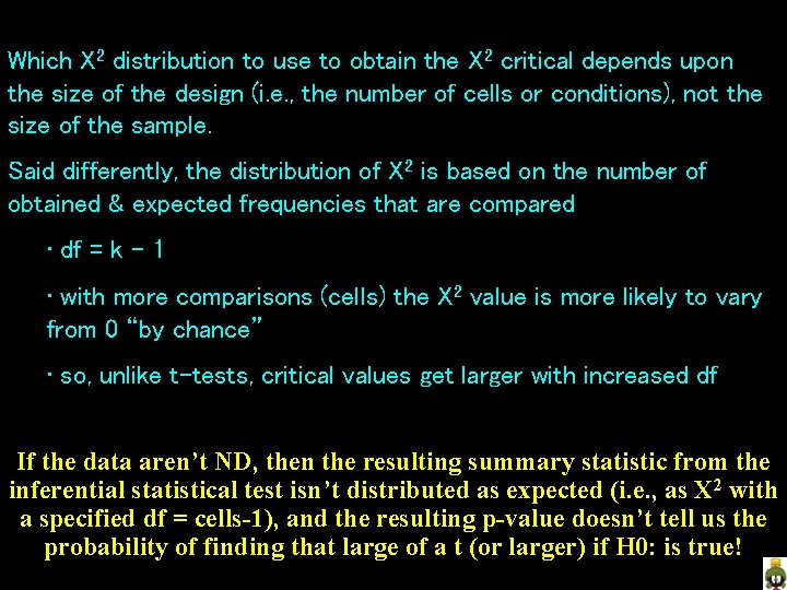
Which X 2 distribution to use to obtain the X 2 critical depends upon the size of the design (i. e. , the number of cells or conditions), not the size of the sample. Said differently, the distribution of X 2 is based on the number of obtained & expected frequencies that are compared • df = k - 1 • with more comparisons (cells) the X 2 value is more likely to vary from 0 “by chance” • so, unlike t-tests, critical values get larger with increased df If the data aren’t ND, then the resulting summary statistic from the inferential statistical test isn’t distributed as expected (i. e. , as X 2 with a specified df = cells-1), and the resulting p-value doesn’t tell us the probability of finding that large of a t (or larger) if H 0: is true!

ANOVA is based on Mean Squares formulas, let’s start there… X 2 = Σ (of – ef)2 ef Remember that a X 2 distribution results from squaring members of a normal distribution Look at the Mean Square formula… Remembering that the mean of a set of scores is the “expected value” of each score – notice the similarity of the numerators of the X 2 and MS formulas? MS = Σ (X – X)2 # -1 • Again, a X 2 distribution will result from squaring members of an ND • So, mean squares are distributed as X 2, with df = # - 1 Of course, once again, if the data aren’t ND, then a X 2 distribution doesn’t result

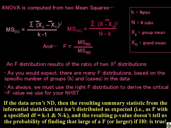
ANOVA is computed from two Mean Squares… MSBG = Σ (Xg – XG)2 k -1 MSWG = And… F = Σ (X - Xg)2 MSBG MSWG N-k k = #grps N = # subs Xg = group mean XG = grand mean An F distribution results of the ratio of two X 2 distributions • As you would expect, there are many F distributions, based on the specific number of groups (k) and (cases) in the data • As always, we must use the right F distribution to derive the critical -F value we use for your NHST If the data aren’t ND, then the resulting summary statistic from the inferential statistical test isn’t distributed as expected (i. e. , as F with a specified df = k-1 & N-k), and the resulting p-value doesn’t tell us the probability of finding that large of a F (or larger) if H 0: is true!

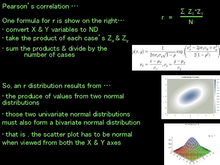
Pearson’s correlation … One formula for r is show on the right… • convert X & Y variables to ND • take the product of each case’s Zx & Zy • sum the products & divide by the number of cases So, an r distribution results from … • the produce of values from two normal distributions • those two univariate normal distributions must also form a bivariate normal distribution • that is , the scatter plot has to be normal when viewed from both the X & Y axes r = Σ ZX*ZY N

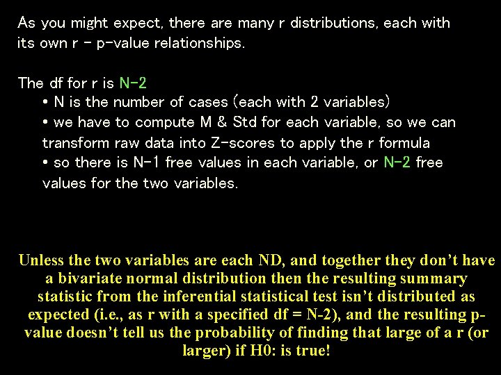
As you might expect, there are many r distributions, each with its own r – p-value relationships. The df for r is N-2 • N is the number of cases (each with 2 variables) • we have to compute M & Std for each variable, so we can transform raw data into Z-scores to apply the r formula • so there is N-1 free values in each variable, or N-2 free values for the two variables. Unless the two variables are each ND, and together they don’t have a bivariate normal distribution the resulting summary statistic from the inferential statistical test isn’t distributed as expected (i. e. , as r with a specified df = N-2), and the resulting pvalue doesn’t tell us the probability of finding that large of a r (or larger) if H 0: is true!