Exploring Assumptions What are assumptions Assumptions are an


- Slides: 27

Exploring Assumptions

What are assumptions? Assumptions are an essential part of statistics and the process of building and testing models. There are many different assumptions across the range of different statistical tests and procedures, but for now we are focusing on several of the most common assumptions and how to check them.

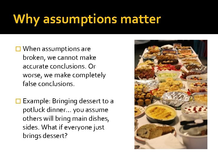
Why assumptions matter � When assumptions are broken, we cannot make accurate conclusions. Or worse, we make completely false conclusions. � Example: Bringing dessert to a potluck dinner… you assume others will bring main dishes, sides. What if everyone just brings dessert?

Assumptions of Parametric Data � Many of the statistical tests that we use in this course are called “parametric” tests. � Many parametric tests are based on the normal distribution. If we use such a test when our data is not, in fact, normal, we will probably get inaccurate estimates. Parametric Statistics: We assume that the data comes from specific class of probability distributions, indexed by a set of parameters. We make inferences about these parameters, selecting a unique distribution as a model for the population.

Four Key Assumptions of Parametric Tests Normally distributed data This can mean different things depending on the context– sometimes we need a population variable to be normally distributed, other times we need the errors in our model to be normally distributed. � Homogeneity of variance Variances should be the same in the data we are using for a given test. So, if we are comparing means between 2, 3 or more groups, we want to know if the variances for each group are different from one another or not. � Interval data That is, equal intervals along the entire range for a given variable. For example, age measured in years is an interval variable. But, age measured in three categories (young, middle aged, old) would not be interval (it is ordinal). � Independence This can also mean many different things, but usually it means that the data from different cases are independent (behavior or action from one case does not influence the behavior or action of another case). �

Assumption of Normality � In many tests we assume that the sampling distribution is normally distributed– but remember that we don’t actually know if the sampling distribution is normally distributed or not. � But we know that if the sample data are approximately normal, then the sampling distribution should also be normal. � Also, by the Central Limit theorem, we know that when we have large sample sizes, then we can be even more confident that the sampling distribution is normally distributed.

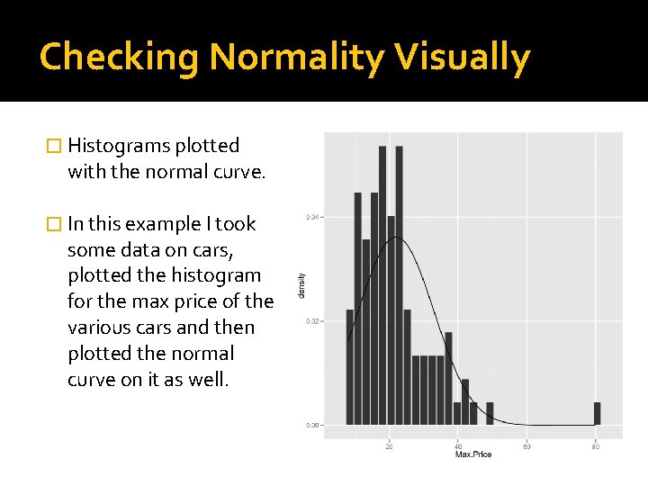
Checking Normality Visually � Histograms plotted with the normal curve. � In this example I took some data on cars, plotted the histogram for the max price of the various cars and then plotted the normal curve on it as well.

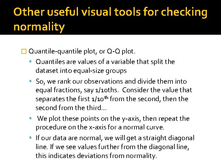
Other useful visual tools for checking normality � Quantile-quantile plot, or Q-Q plot. Quantiles are values of a variable that split the dataset into equal-size groups So, we rank our observations and divide them into equal fractions, say 1/10 ths. Consider the value that separates the first 1/10 th from the second, then the second from the third… We plot these points on the y-axis, then repeat the procedure on the x-axis for a normal curve. If our data are normal, we will get a straight diagonal line. If we see values further from the diagonal line, this indicates deviations from normality.

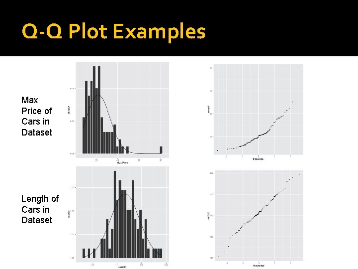
Q-Q Plot Examples Max Price of Cars in Dataset Length of Cars in Dataset

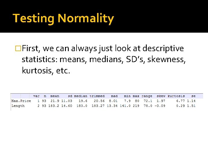
Testing Normality �First, we can always just look at descriptive statistics: means, medians, SD’s, skewness, kurtosis, etc.

Shapiro-Wilk test �We can also conduct a Shapiro-Wilk test, which compares the scores in the sample to a normally distributed set of scores. Null hypothesis = the distribution of the sample is the same as a normal distribution. Alt hypothesis = the distribution of the sample is not the same as a normal distribution. ▪ Thus, if we find a significant p-value (e. g, p <. 05) then this means that we have a non-normal distribution.

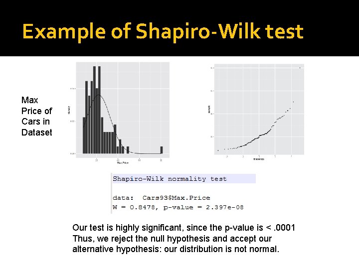
Example of Shapiro-Wilk test Max Price of Cars in Dataset Our test is highly significant, since the p-value is <. 0001 Thus, we reject the null hypothesis and accept our alternative hypothesis: our distribution is not normal.

Interpreting a Shapiro-Wilk test High P-value Low P-value We have a normal distribution <or> Just not enough data to reject the hypothesis of normality Our distribution is very non-normal <or> Our distribution is slightly non-normal, but we have so much data we can reject the normal hypothesis anyway

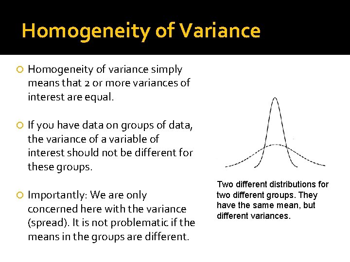
Homogeneity of Variance Homogeneity of variance simply means that 2 or more variances of interest are equal. If you have data on groups of data, the variance of a variable of interest should not be different for these groups. Importantly: We are only concerned here with the variance (spread). It is not problematic if the means in the groups are different. Two different distributions for two different groups. They have the same mean, but different variances.

Testing Homogeneity of Variance �Levene’s Test: Allows us to examine whether the variances between groups are different or not. Null hypothesis = the variances for the groups are equal. Alt hypothesis = the variances for the groups are not equal. ▪ Thus, if we find a significant p-value (e. g, p <. 05) then this means that we have unequal variances between groups.

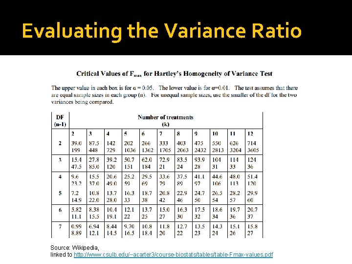
Testing Homogeneity of Variance in Large Samples �Levene’s test is often significant when you have a very large sample of data. �Hartley’s Fmax (or, variance ratio) is a ratio between the group with the largest variance and the group with smallest variance.

Evaluating the Variance Ratio Source: Wikipedia, linked to http: //www. csulb. edu/~acarter 3/course-biostats/table-Fmax-values. pdf

In sum… �It is useful to look at both the variance ratio and Levene’s test when you are using very large data. �We will return to using and applying test of homogeneity of variance as we work with statistical tests that rely on this assumption.

Correcting Problems with Data There are two procedures that we can use to directly correct problems in a given dataset: Outliers ▪ An observation that is numerically distinct from the rest of the data. ▪ Example: survey of undergraduate majors that lead to highest incomes. Transforming Data ▪ Used when we need to meet the assumptions of a normal distribution in order to conduct a particular statistical test, but we have failed the assumption of normality (e. g. , Shapiro-Wilk test)

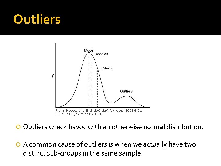
Outliers From: Hedges and Shah BMC Bioinformatics 2003 4: 31 doi: 10. 1186/1471 -2105 -4 -31 Outliers wreck havoc with an otherwise normal distribution. A common cause of outliers is when we actually have two distinct sub-groups in the sample.

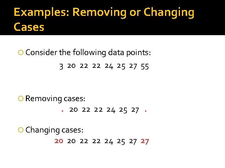
Dealing with Outliers � Removing the case(s). This is also called “trimming”. Quite literally, deleting the case (or hiding the case) so that it is not part of any analysis that you conduct. You have to be able to justify this decision– we cannot just delete cases because they do not ‘fit’ what we expect. The key issue is whether the outliers are actually very different from the rest of the sample. Common reasons for removing/trimming: ▪ Data is out of range, perhaps due to data entry error (scale is 1 -100, value is 200) ▪ Measurement error (something in our measurement appears to produce incorrect values for some cases).

Dealing with Outliers (continued) Changing the value of the case Essentially we replace the outlier cases with some other value. For example, assign the next highest or lowest value in the sample that is not an outlier. For fairly obvious reasons, this is usually the least preferred option.

Examples: Removing or Changing Cases Consider the following data points: 3 20 22 22 24 25 27 55 Removing cases: . 20 22 22 24 25 27. Changing cases: 20 20 22 22 24 25 27 27

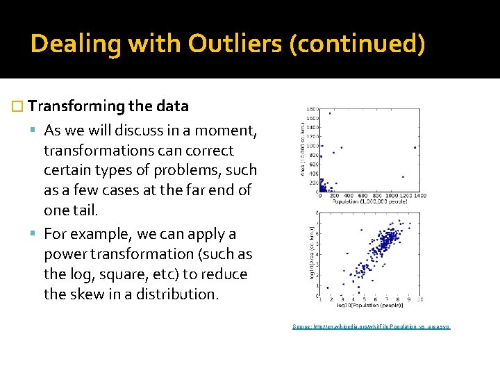
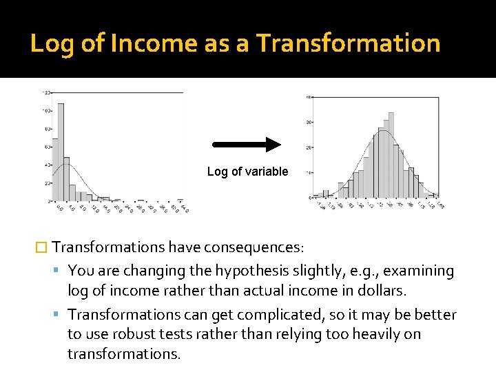
Dealing with Outliers (continued) � Transforming the data As we will discuss in a moment, transformations can correct certain types of problems, such as a few cases at the far end of one tail. For example, we can apply a power transformation (such as the log, square, etc) to reduce the skew in a distribution. Source: http: //en. wikipedia. org/wiki/File: Population_vs_area. svg

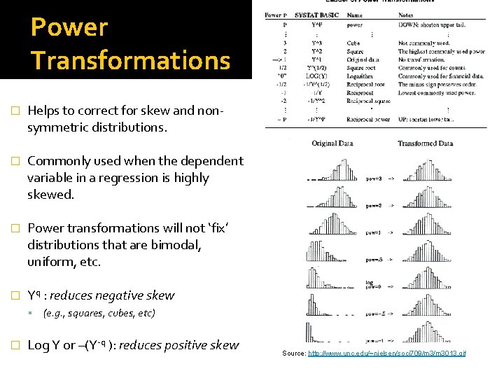
Power Transformations � Helps to correct for skew and nonsymmetric distributions. � Commonly used when the dependent variable in a regression is highly skewed. � Power transformations will not ‘fix’ distributions that are bimodal, uniform, etc. � Yq : reduces negative skew (e. g. , squares, cubes, etc) � Log Y or –(Y-q ): reduces positive skew Source: http: //www. unc. edu/~nielsen/soci 709/m 3013. gif

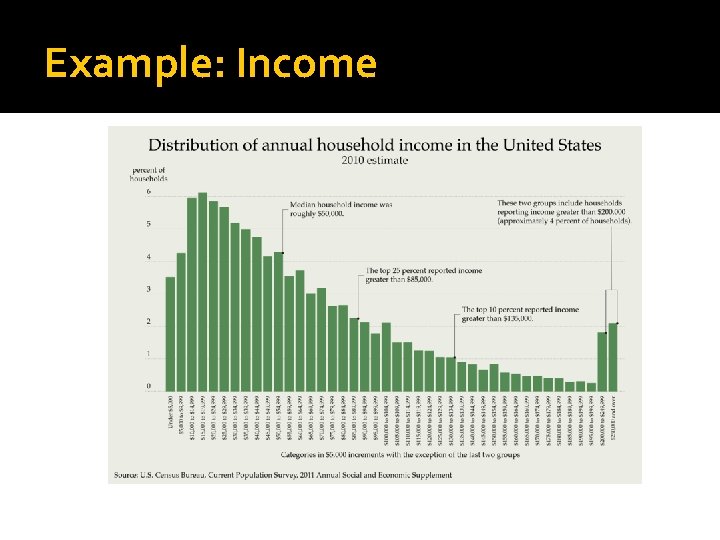
Example: Income

Log of Income as a Transformation Log of variable � Transformations have consequences: You are changing the hypothesis slightly, e. g. , examining log of income rather than actual income in dollars. Transformations can get complicated, so it may be better to use robust tests rather than relying too heavily on transformations.