Anisotropic Diffusion Summing of the article scalespace and

Anisotropic Diffusion Summing of the article “scale-space and edge detection using anisotropic diffusion” By Pietro Perona And Jitendra Malik Nerya Agam Computer-Science undergraduate

About the upcoming class: • In this class, we will introduce the basics of Anisotropic diffusion, and its usage in scale-space actions and edge detection in graphic images. • The focus of the lecture will be gaining intuition about the Anisotropic Diffusion work process. Less focus will be dedicated to Mathematical analysis of procedures. This author thereby promises, to make his best effort and keep you interested throughout the class. • Any attendant may ask any question at any time during class.

Introduction What is the main drawback of this picture ? -Image noise In what ways does it bother us ? - visually… as humans - lost detail - renders the image unfit for most of our desired image manipulation filters

So, we are looking for an efficient method of noise removal, that is able to clarify the image.

Methods of noise removal were known a long time before the Anisotropic Diffusion case was first claimed (1990) Most of the methods are typically forms of applying a blur filter to the image, as Blurring it hopefully results in a smooth, noise-less product. Such a product, with low noise levels, is a much better starting point for any image related algorithm…

Classic smoothing methods: • Based on convolving a Gaussian kernel with each and every pixel. A typical kernel would be of size Nx. N. • The single pixel’s brightness value is determined by its own original value, as well as the values of its neighbor pixels. • an appropriate definition of the transformation would be: I (x, y) = I 0 (x, y) * G(x, y, t)

Making a gaussian kernel of size Nx. N: • Set the center of the kernel to be x=0, y=0 => (0, 0) • Using the equation, set the values on every square of the kernel: Squares closer to the center (such as (1, 2)) would get higher values than squares which are close to the kernel’s border. Note: t = theoretically is sigma^2, tough – in a C. s implementation it is the size of the gaussian (3 x 3, 7 x 7 etc…)

Gaussian 5 x 5 (without normalization) 2 4 5 4 2 4 9 12 9 4 5 12 15 12 5 4 9 12 9 4 2 4 5 4 2

Taking a gaussian kernel of size Nx. N: • Set the center of the kernel to be x=0, y=0 => (0, 0) • Using the equation, set the values on every square of the kernel: Squares closer to the center (such as (1, 2)) would get higher values than squares which are close to the kernel’s border. The parameter t stands for the variance of the gaussian: when t=0 => I(x, y) = I 0(x, y) (just the ID transform…) As t grows, the brightness of a pixel in the resulting image considers more and more of its neighboring values.

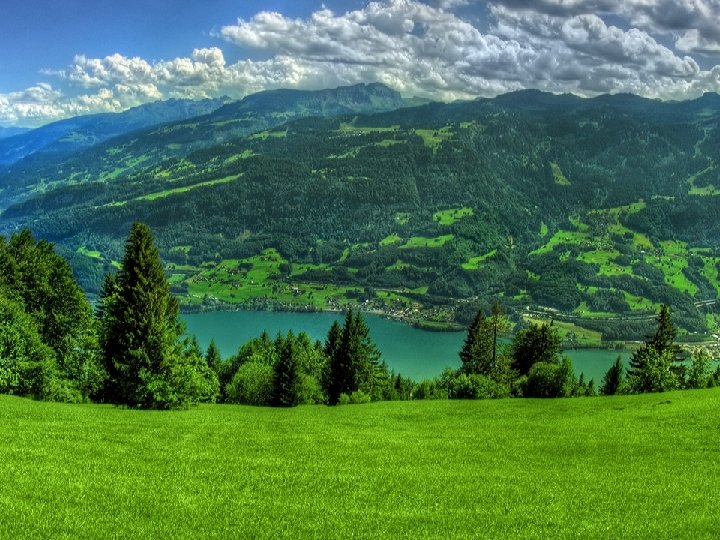
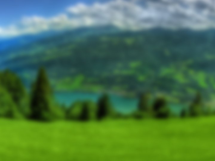
In this next example, notice how the blurring makes the grass color almost completely homogeneous… which in our case is considered a desired effect. This is because the smoothing operation is vary useful in highly homogeneous regions, since it scales-down the complexity of the region to a simple “blub” of very few discrete brightness levels. Using a few iterations of classic Gaussian Blurring, with kernel size of 7 x 7, 9 x 9 and 13 x 13, gives the following product image:

While being a popular tool, Gaussian pass has its downsides: • Loss of fine detail • Smoothing across boundaries The first could be expected, as it is the direct trade-off of smoothing … The second is problematic – with no clear boundaries, image segmentation proves to be difficult. Here are some examples:

This ww 2 photo is given here in its original form. From a human eye point of view – it has a good enough quality. Pay attention : some surfaces, like the runway’s asphalt or the roofs of the buildings, do not have a smooth texture… (pacific us navy airbase, ww 2)

Now, pass the airbase photo through an edge detecting filter (sobel). Result: along with the “correct” edges, this product photo contains many false edges. This is not a good enough edge -marking product.

If we smooth the image, we can expect a lot less noise… Smoothing the original with Gaussian 5 x 5…

Running edge detection… Many of the false edges were smoothed. Unfortunately, so were the true edges.

Using this linear smoothing, gives especially poor results in more coarse images (a. k. a low resolution images), as Blurring already makes an image a lot more coarse. This is because meaningful edges in a coarse image would be smudged so much, that it is hard to determine where the real meaningful edge is originally located.

Perona & Malik suggestion

Perona & Malik suggestion A smoothing algorithm has to stand to a criteria: 1. Causality – no spurious detail should be generated while passing from finer to coarser scales. 2. Immediate Localization – at each resolution, the region boundaries should be sharp and coincide with the “semantically meaningful” boundaries at that resolution. 3. Piecewise Smoothing – at all scales, intraregion smoothing should occur preferentially over interregion smoothing. Smoothing that respects this criteria should get better results…

Maybe as good as this: Maybe better… ?

In order to achieve this desired filtering, lets take a look at some of the basic fundamentals, that compose the whole algorithm… Starting with: Non-Linear passes

Linear approach: Treat every pixel with the exact same convolution. Non-Linear approach: Treat a pixel with varying intensity, depending on its neighborhood qualities.

Here is an abstraction of the principal: A Non-Linear equation, helpful to our cause… Let us say that we have a method “E” of knowing if a certain point in the image is a part of an edge or not. We can make a new transformation… a filter that smoothes inside a region, but “skips” the edges in the image. Generally speaking: if (x, y) is a part of an edge apply little smoothing if not a part of an edge apply full smoothing

To implement this specific Non-Linear approach, we need a detector to tell us if (x, y) is a part of an edge or not. Luckily, the Gradient of the brightness function is quite good for that:

In the first part, the gradient vector is (0, n) while (n > 0) In the second part, the gradient vector is (-m , m) while (m > 0 ) These points where the norm of the gradient is high, could be treated as “edge points”, end therefore be applied less blurring…

The coefficient Until now: We have an edge/not edge estimation method “E”. We need to create a function “g”, that controls blurring intensity according to. “g” has to be a monotonous decreasing function (why ? )

The coefficient Perona & Malik trialed with two different “g” definitions:

K=1 K=4

The coefficient Now, we have E and g. Let us define the coefficient. The coefficient controls how much smoothing is done in (x, y) Simplification: - C(x, y, t) is large when x, y is not a part of an edge - C(x, y, t) is small when x, y, is a part of an edge

Original Linear Non-Linear

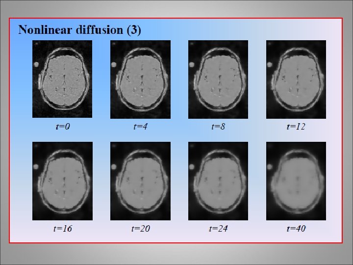
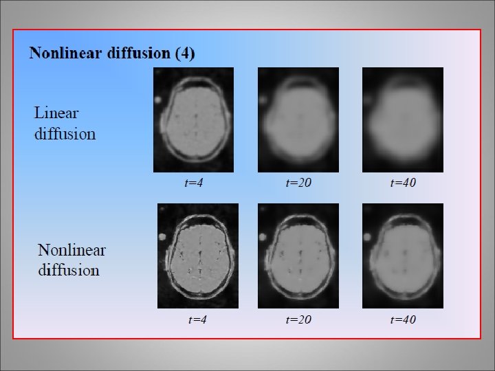
A Non-Linear pass has these properties: • Good intraregion smoothing • generally keeps the edges as they were, doesn’t do much interregion smoothing So, going Non-Linear might be a part of the solution, but is not good enough on its own… (edges stay rough) Continuing with: Anisotropic Diffusion

Warning: The following may strengthen your intuition of the flow of a smoothing process

Diffusion describes the spread of particles through random motion from regions of higher concentration to regions of lower concentration. (wiki)

• Isotropic: that is not dependent of direction. • Anisotropic: depends on the direction applied

Koenderink and Hummel pointed out that the family (family = product of different t values) of derived images from the equation: I (x, y) = I 0 (x, y) * G (x, y, t) Can be viewed as: the solution of the Heat Diffusion equation

Like heat, generated in a cold surrounding… the gradient size represents the margins of temperature. As time advances on (t), each potent molecule (a “hot” unit) spreads in the direction of its gradient vector. Surprisingly, it is also valid for liquid diffusion… and more. The matter in an image is not heat, but brightness level… So, an image could be generalized to be a surface, where bright spots are “hot” and dark spots are “cold”. spreading is explained by Fick’s law, were J is the quantity of matter flowing through a “check point” x. this is beyond this class’s scope

Heat spread Do you get the intuition ?

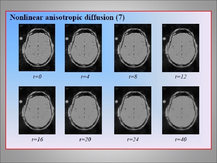
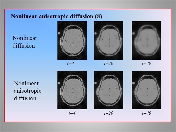
Anisotropic approach Wanted: A form of smoothing specifically edges, with out loosing significance. If found: Then it could be combined with the non-linear smoothing idea, to produce an “all around” smoothing filter. Remember – main drawback of the non-linear approach we saw earlier, was lack of intra-edge smoothing. Ideas ?

Use varying smoothing kernels !

The desired “direction” of the dynamic kernel is effected by the local gradient’s direction. It is perpendicular to it… If gradient is (a, b), then a perpendicular vector to it, can be (a, -b) A dynamic kernel is contracted along the direction of the normal, ending in an elipticall kernel.

Original Anisotropic Diffusion

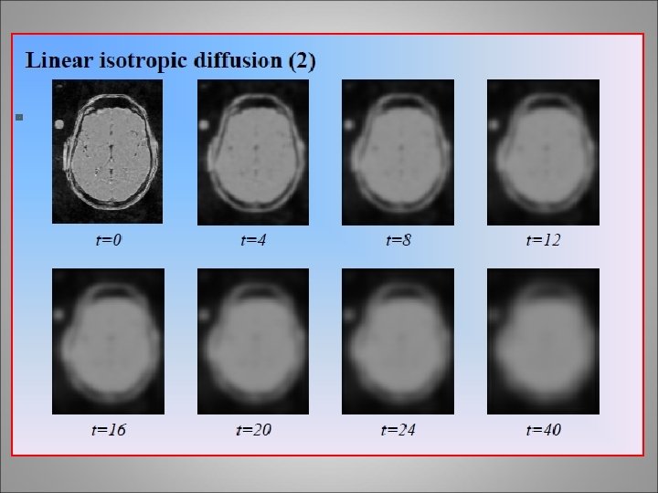
Original Linear isotropic diffusion (simple gaussian)

Original Non-linear isotropic diffusion (edge skipping)

Original Non-linear anisotropic diffusion

If there is someone among this crowd who still has doubt in his heart, he may speak now