Recent Progress in the Design and Analysis of

Recent Progress in the Design and Analysis of Admissible Heuristic Functions Richard E. Korf Computer Science Department University of California, Los Angeles

Thanks • • • Victoria Cortessis Ariel Felner Rob Holte Kaoru Mulvihill Nathan Sturtevant

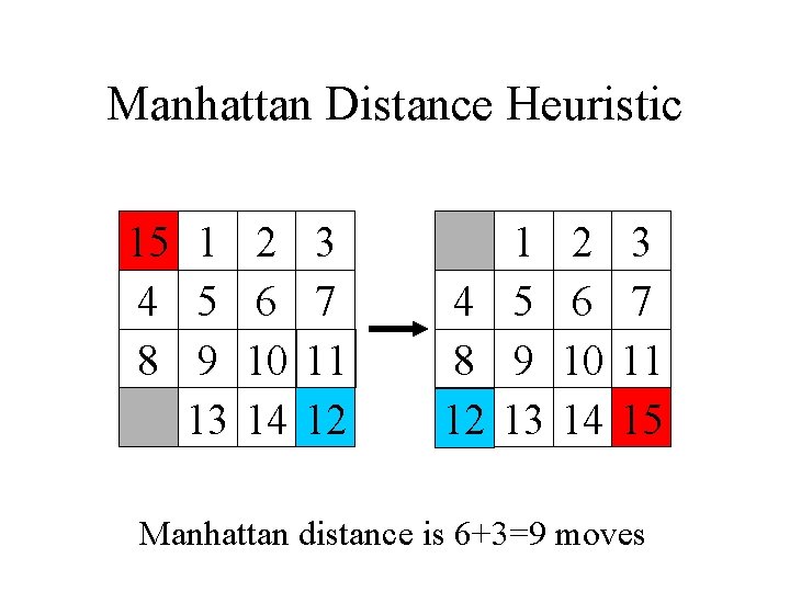
Heuristics come from Abstractions • Admissible (lower bound) heuristic evaluation functions are often the cost of exact solutions to abstract problems. • E. g. If we relax the Fifteen Puzzle to allow a tile to move to any adjacent position, the cost of an exact solution to this simplified problem is Manhattan distance.

Outline of Talk • New methods for the design of more accurate heuristic evaluation functions. • A new method to predict the running time of admissible heuristic search algorithms

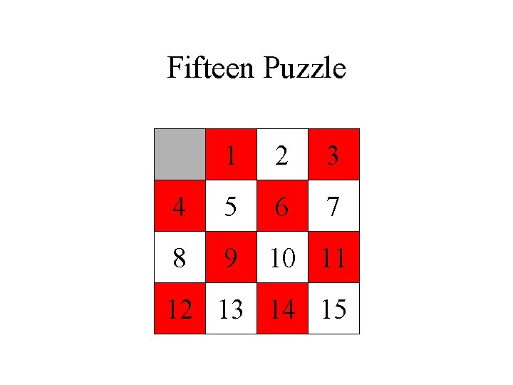
Fifteen Puzzle 1 2 3 4 5 6 7 8 9 10 11 12 13 14 15

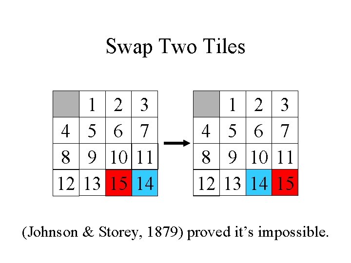
Fifteen Puzzle • Invented by Sam Loyd in 1870 s • “. . . engaged the attention of nine out of ten persons of both sexes and of all ages and conditions of the community. ” • $1000 prize to swap positions of two tiles

Swap Two Tiles 1 4 5 8 9 12 13 2 6 10 15 3 7 11 14 1 4 5 8 9 12 13 2 6 10 14 3 7 11 15 (Johnson & Storey, 1879) proved it’s impossible.

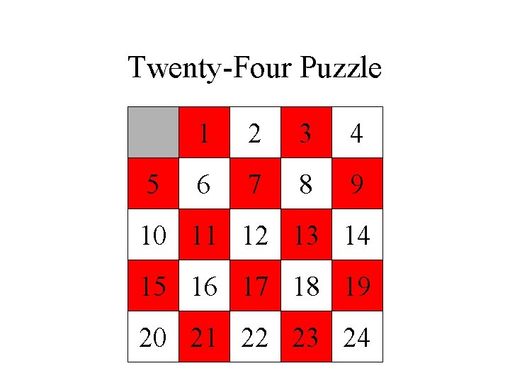
Twenty-Four Puzzle 5 1 2 3 4 6 7 8 9 10 11 12 13 14 15 16 17 18 19 20 21 22 23 24

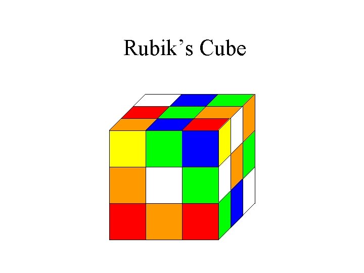
Rubik’s Cube

Rubik’s Cube • Invented in 1974 by Erno Rubik of Hungary • Over 100 million sold worldwide • Most famous combinatorial puzzle ever

Finding Optimal Solutions • Input: A random solvable initial state • Output: A shortest sequence of moves that maps the initial state to the goal state • Generalized sliding-tile puzzle is NP Complete (Ratner and Warmuth, 1986) • People can’t find optimal solutions. • Progress measured by size of problems that can be solved optimally.

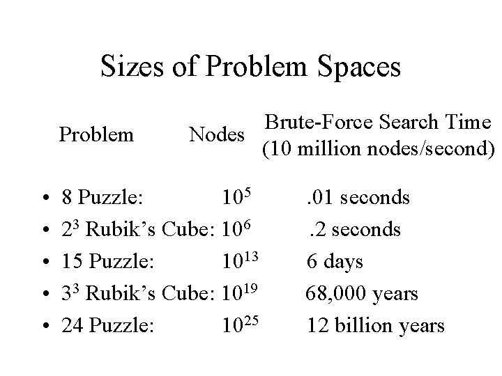
Sizes of Problem Spaces Problem • • • Brute-Force Search Time Nodes (10 million nodes/second) 8 Puzzle: 105 23 Rubik’s Cube: 106 15 Puzzle: 1013 33 Rubik’s Cube: 1019 24 Puzzle: 1025 . 01 seconds. 2 seconds 6 days 68, 000 years 12 billion years

A* Algorithm • Hart, Nilsson, and Raphael, 1968 • Best-first search with cost function f(n)=g(n)+h(n) • If h(n) is admissible (a lower bound estimate of optimal cost), A* guarantees optimal solutions if they exist. • A* stores all the nodes it generates, exhausting available memory in minutes.

Iterative-Deepening-A* (IDA*) • IDA* (Korf, 1985) is a linear-space version of A*, using the same cost function. • Each iteration searches depth-first for solutions of a given length. • IDA* is simpler, and often faster than A*, due to less overhead per node. • Key to performance is accurate heuristic evaluation function.

Manhattan Distance Heuristic 15 1 2 3 4 5 6 7 8 9 10 11 13 14 12 1 4 5 8 9 12 13 2 6 10 14 3 7 11 15 Manhattan distance is 6+3=9 moves

Performance on 15 Puzzle • Random 15 puzzle instances were first solved optimally using IDA* with Manhattan distance heuristic (Korf, 1985). • Optimal solution lengths average 53 moves. • 400 million nodes generated on average. • Average solution time is about 50 seconds on current machines.

Limitation of Manhattan Distance • To solve a 24 -Puzzle instance, IDA* with Manhattan distance would take about 65, 000 years on average. • Assumes that each tile moves independently • In fact, tiles interfere with each other. • Accounting for these interactions is the key to more accurate heuristic functions.

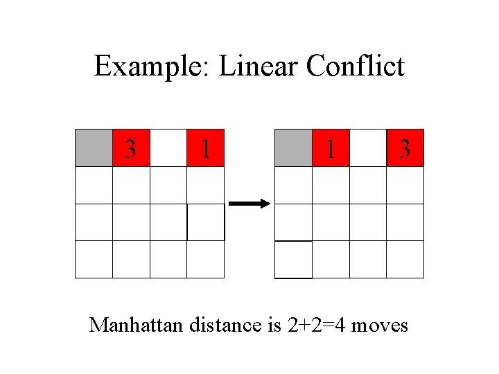
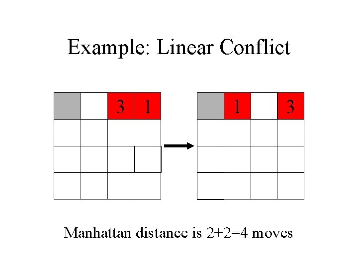
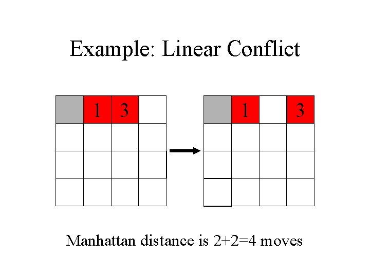
Example: Linear Conflict 3 1 1 3 Manhattan distance is 2+2=4 moves

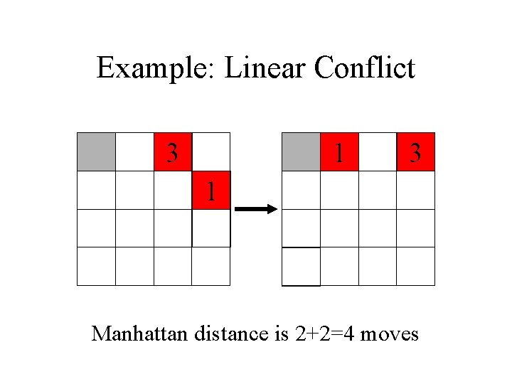
Example: Linear Conflict 3 1 1 3 Manhattan distance is 2+2=4 moves

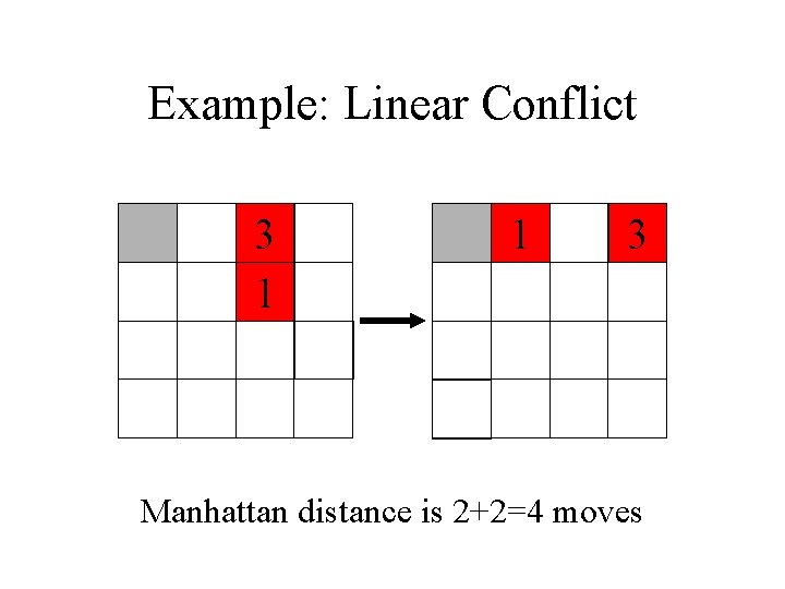
Example: Linear Conflict 3 1 Manhattan distance is 2+2=4 moves

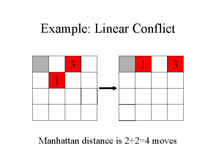
Example: Linear Conflict 3 1 1 3 Manhattan distance is 2+2=4 moves

Example: Linear Conflict 3 1 Manhattan distance is 2+2=4 moves

Example: Linear Conflict 1 3 Manhattan distance is 2+2=4 moves

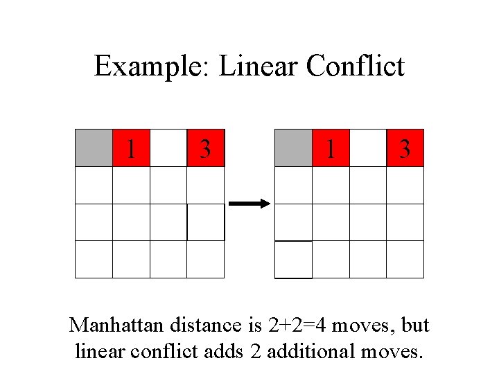
Example: Linear Conflict 1 3 Manhattan distance is 2+2=4 moves, but linear conflict adds 2 additional moves.

Linear Conflict Heuristic • Hansson, Mayer, and Yung, 1991 • Given two tiles in their goal row, but reversed in position, additional vertical moves can be added to Manhattan distance. • Still not accurate enough to solve 24 -Puzzle • We can generalize this idea further.

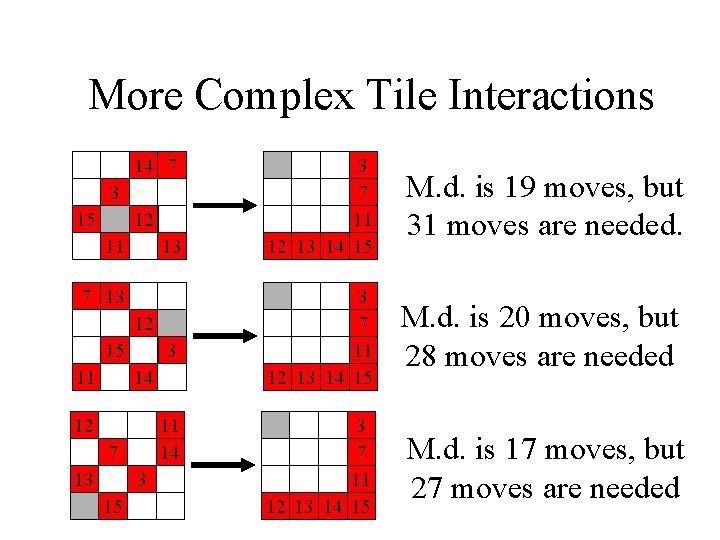
More Complex Tile Interactions 14 7 3 15 12 11 13 7 13 12 15 11 3 14 12 11 14 7 13 3 15 3 7 11 12 13 14 15 M. d. is 19 moves, but 31 moves are needed. 3 7 11 12 13 14 15 M. d. is 20 moves, but 28 moves are needed 3 7 11 12 13 14 15 M. d. is 17 moves, but 27 moves are needed

Pattern Database Heuristics • Culberson and Schaeffer, 1996 • A pattern database is a complete set of such positions, with associated number of moves. • e. g. a 7 -tile pattern database for the Fifteen Puzzle contains 519 million entries.

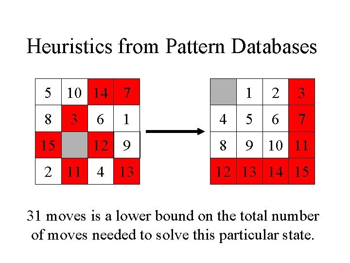
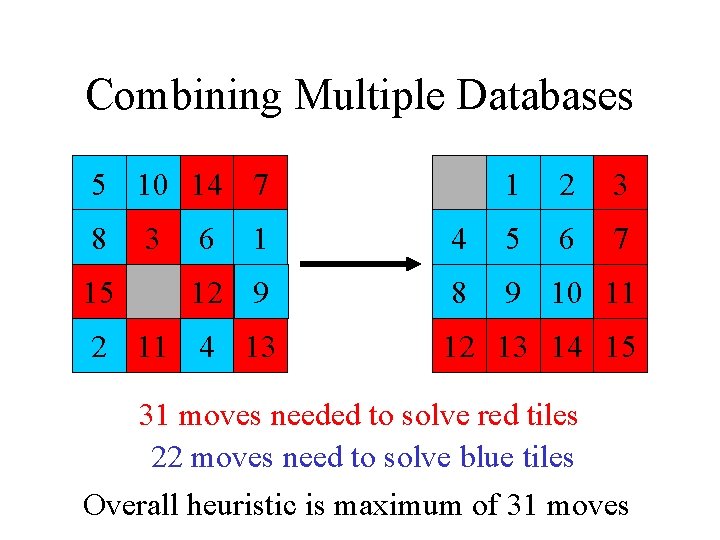
Heuristics from Pattern Databases 5 10 14 7 8 15 3 6 1 2 3 6 7 1 4 5 12 9 8 9 10 11 2 11 4 13 12 13 14 15 31 moves is a lower bound on the total number of moves needed to solve this particular state.

Precomputing Pattern Databases • Entire database is computed with one backward breadth-first search from goal. • All non-pattern tiles are indistinguishable, but all tile moves are counted. • The first time each state is encountered, the total number of moves made so far is stored. • Once computed, the same table is used for all problems with the same goal state.

What About the Non-Pattern Tiles? • Given more memory, we can compute additional pattern databases from the remaining tiles. • In fact, we can compute multiple pattern databases from overlapping sets of tiles. • The only limit is the amount of memory available to store the pattern databases.

Combining Multiple Databases 5 10 14 7 8 15 3 6 1 2 3 6 7 1 4 5 12 9 8 9 10 11 2 11 4 13 12 13 14 15 31 moves needed to solve red tiles 22 moves need to solve blue tiles Overall heuristic is maximum of 31 moves

Applications of Pattern Databases • On 15 puzzle, IDA* with pattern database heuristics is about 10 times faster than with Manhattan distance (Culberson and Schaeffer, 1996). • Pattern databases can also be applied to Rubik’s Cube.

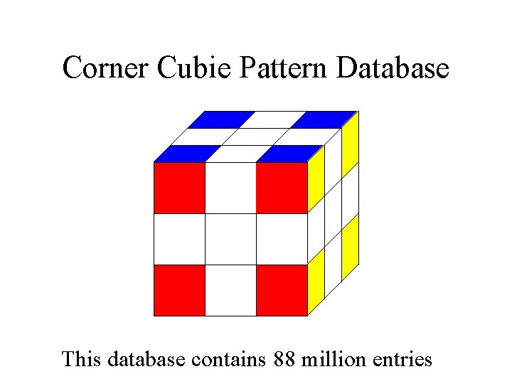
Corner Cubie Pattern Database This database contains 88 million entries

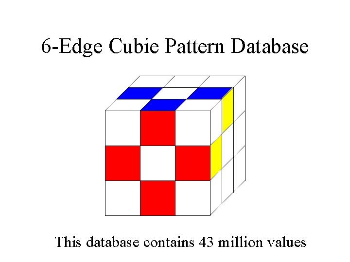
6 -Edge Cubie Pattern Database This database contains 43 million values

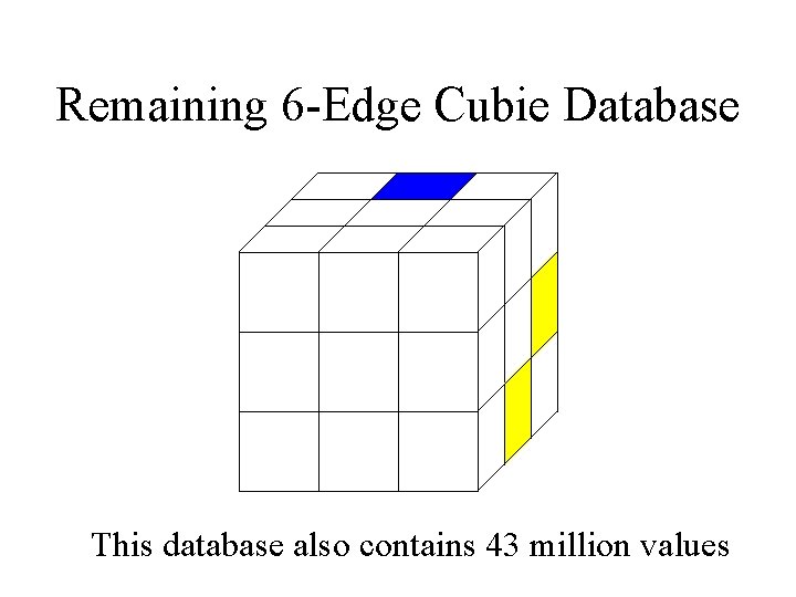
Remaining 6 -Edge Cubie Database This database also contains 43 million values

Rubik’s Cube Heuristic • All three databases are precomputed in less than an hour, and use less than 100 Mbytes. • During problem solving, for each state, the different sets of cubies are used to compute indices into their pattern databases. • The overall heuristic value is the maximum of the three different database values.

Performance on Rubik’s Cube • IDA* with this heuristic found the first optimal solutions to randomly scrambled Rubik’s Cubes (Korf, 1997). • Median optimal solution length is 18 moves • Most problems can be solved in about a day now, using larger pattern databases.

Related Work • Culberson and Schaeffer’s 1996 work on pattern databases in the Fifteen Puzzle. • Armand Prieditis’ ABSOLVER program discovered a “center-corner” heuristic for Rubik’s Cube in 1993. • Herbert Kociemba independently developed a powerful Rubik’s Cube program in 1990 s. • Mike Reid has built faster Cube programs.

Memory Adds Speed • More memory can hold larger databases. • Larger databases provide more accurate heuristic values. • More accurate heuristics speed up search. • E. g. Doubling the memory almost doubles the search speed. • See (Holte and Hernadvolgyi, 1999, 2000) for more details.

Limitation of General Databases • The only way to admissibly combine values from multiple general pattern databases is to take the maximum of their values. • For more accuracy, we would like to add heuristic values from different databases. • We can do this on the tile puzzles because each move only moves one tile at a time. • Joint work with Ariel Felner

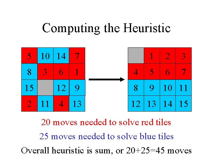
Additive Pattern Databases • Culberson and Schaeffer counted all moves needed to correctly position the pattern tiles. • In contrast, we count only moves of the pattern tiles, ignoring non-pattern moves. • If no tile belongs to more than one pattern, then we can add their heuristic values. • Manhattan distance is a special case of this, where each pattern contains a single tile.

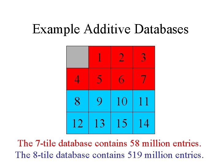
Example Additive Databases 1 2 3 4 5 6 7 8 9 10 11 12 13 15 14 The 7 -tile database contains 58 million entries. The 8 -tile database contains 519 million entries.

Computing the Heuristic 5 10 14 7 8 15 3 6 1 2 3 6 7 1 4 5 12 9 8 9 10 11 2 11 4 13 12 13 14 15 20 moves needed to solve red tiles 25 moves needed to solve blue tiles Overall heuristic is sum, or 20+25=45 moves

Performance on 15 Puzzle • IDA* with a heuristic based on these additive pattern databases can optimally solve random 15 puzzle instances in less than 29 milliseconds on average. • This is about 1700 times faster than with Manhattan distance on the same machine.

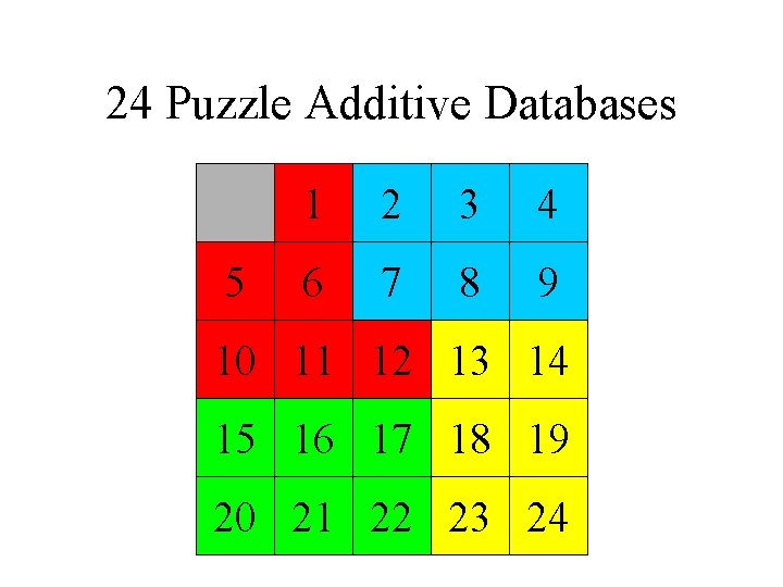
24 Puzzle Additive Databases 5 1 2 3 4 6 7 8 9 10 11 12 13 14 15 16 17 18 19 20 21 22 23 24

Performance on 24 Puzzle • Each database contains 128 million entries. • IDA* using these databases can optimally solve random 24 -puzzle problems. • Optimal solutions average 100 moves. • Billions to trillions of nodes generated. • Over 2 million nodes per second. • Running times from 18 seconds to 10 days. • Average is a day and a half.

Moral of the Story (so far) • Our implementation of disjoint additive pattern databases is tailored to tile puzzles. • In general, most heuristics assume that subproblems are independent. • Capturing some of the interactions between subproblems yields more accurate heuristics • We’ve also applied this to graph partioning.

Time Complexity of Admissible Heuristic Search Algorithms Joint work with Michael Reid (Brown University)

Previous Work on This Problem • Pohl 1977, Gaschnig 1979, Pearl 1984 • Assumes an abstract analytic model of the problem space • Characterizes heuristic by its accuracy as an estimate of optimal solution cost • Produces asymptotic results. • Doesn’t predict runtime on real problems.

How Long does a Heuristic Search Algorithm take to Run? Depends on: • Branching factor of problem space • Solution depth of problem instance • Heuristic evaluation function

Branching Factor: average number of children of a node • In tile puzzles, a cell has 2, 3, or 4 neighbors. • Eliminating inverse of last move gives a node branching factor of 1, 2, or 3. • Exact asymptotic branching factor depends on relative frequency of each type of node, in limit of large depth. • Joint work with Stefan Edelkamp

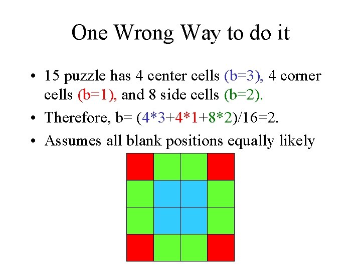
One Wrong Way to do it • 15 puzzle has 4 center cells (b=3), 4 corner cells (b=1), and 8 side cells (b=2). • Therefore, b= (4*3+4*1+8*2)/16=2. • Assumes all blank positions equally likely

The Correct Answer • The asymptotic branching factor of the Fifteen Puzzle is 2. 13040 • The derivation is left as an exercise.

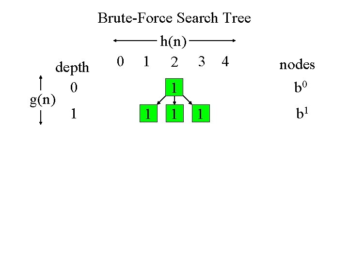
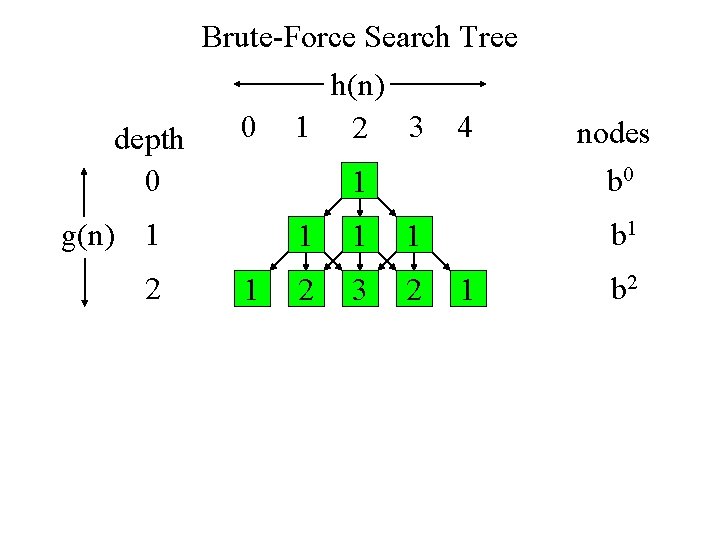
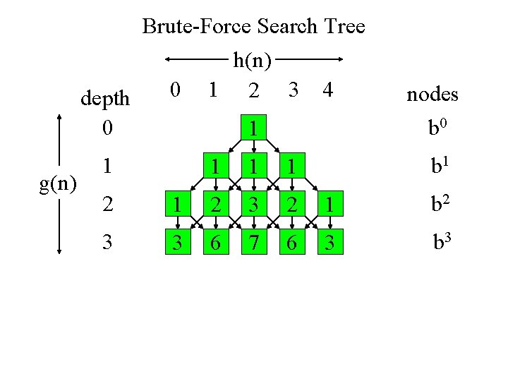
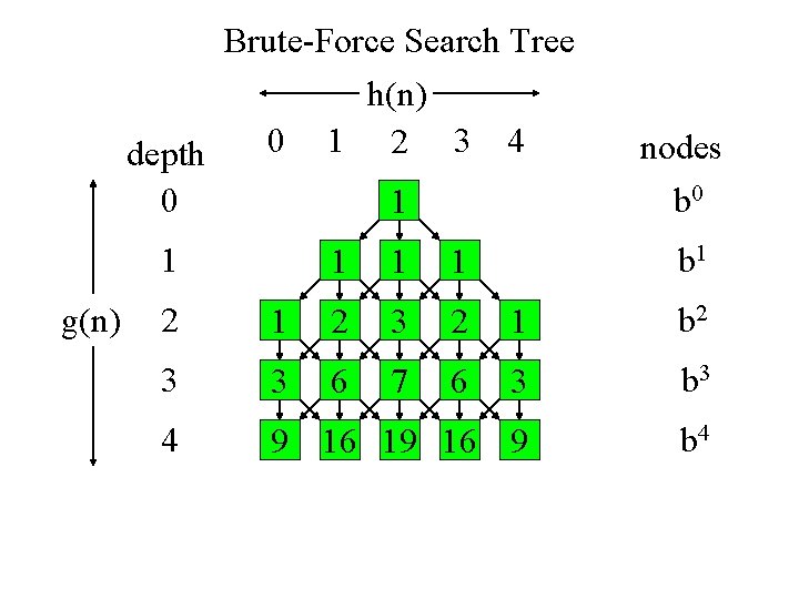
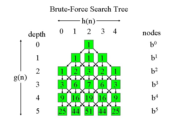
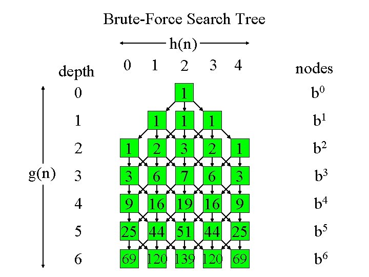
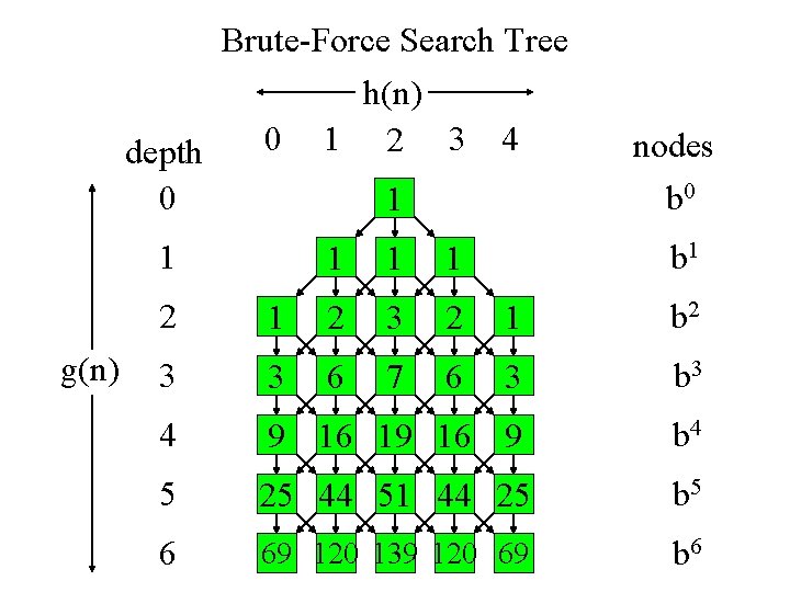
Derivation of Time Complexity • First, consider brute-force search. • Then, consider heuristic search complexity. • Illustrate result with example search tree.

Brute-Force Search Tree h(n) 0 1 2 3 4 depth 0 1 g(n) 1 1 nodes b 0 b 1

Brute-Force Search Tree h(n) 0 1 2 3 4 depth 0 1 g(n) 1 2 1 1 2 3 2 nodes b 0 b 1 1 b 2

Brute-Force Search Tree h(n) 0 1 2 3 4 depth 0 1 g(n) 1 1 nodes b 0 b 1 2 3 2 1 b 2 3 3 6 7 6 3 b 3

Brute-Force Search Tree h(n) 0 1 2 3 4 depth 0 1 1 g(n) 1 1 1 nodes b 0 b 1 2 3 2 1 b 2 3 3 6 7 6 3 b 3 4 9 16 19 16 9 b 4

Brute-Force Search Tree h(n) 0 1 2 3 4 depth 0 1 1 g(n) 1 1 1 nodes b 0 b 1 2 3 2 1 b 2 3 3 6 7 6 3 b 3 4 9 16 19 16 9 b 4 5 25 44 51 44 25 b 5

Brute-Force Search Tree h(n) 0 1 2 3 4 depth 0 1 1 g(n) 1 1 1 nodes b 0 b 1 2 3 2 1 b 2 3 3 6 7 6 3 b 3 4 9 16 19 16 9 b 4 5 25 44 51 44 25 b 5 6 69 120 139 120 69 b 6

Heuristic Distribution Function • The distribution of heuristic values converges, independent of initial state. • Let P(x) be the proportion of states with heuristic value <= x, in limit of large depth. • For pattern database heuristics, P(x) can be computed exactly from the databases. • For general heuristics, P(x) can be approximated by random sampling.

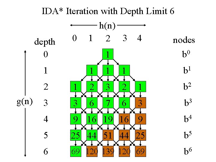
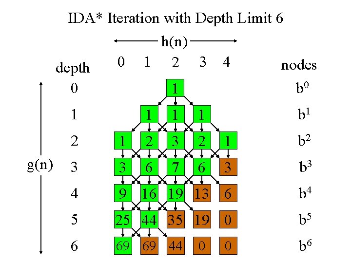
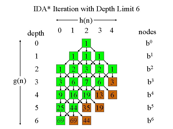
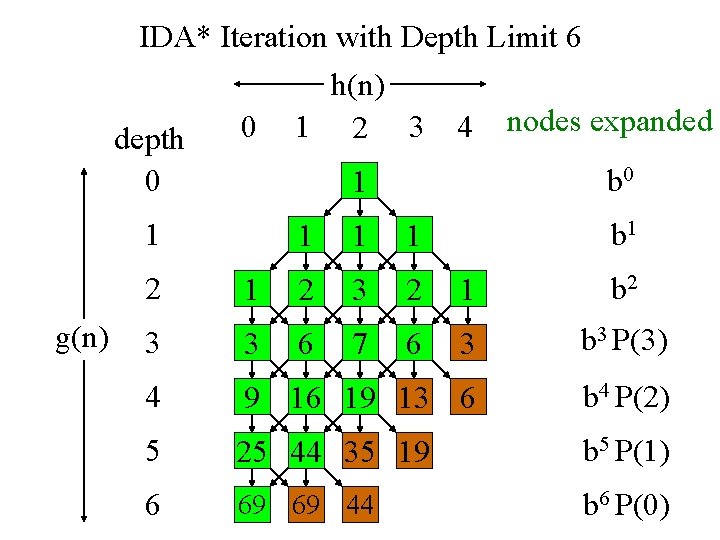
Nodes Expanded by A* or IDA* • Running time is proportional to number of node expansions. • If C* is the cost of an optimal solution, A* or IDA* will expand all nodes n for which f(n)=g(n)+h(n)<=C*, in the worst case.

Brute-Force Search Tree h(n) 0 1 2 3 4 depth 0 1 1 g(n) 1 1 1 nodes b 0 b 1 2 3 2 1 b 2 3 3 6 7 6 3 b 3 4 9 16 19 16 9 b 4 5 25 44 51 44 25 b 5 6 69 120 139 120 69 b 6

IDA* Iteration with Depth Limit 6 h(n) 0 1 2 3 4 nodes depth 0 b 0 1 1 g(n) 1 1 1 b 1 2 3 2 1 b 2 3 3 6 7 6 3 b 3 4 9 16 19 16 9 b 4 5 25 44 51 44 25 b 5 6 69 120 139 120 69 b 6

IDA* Iteration with Depth Limit 6 h(n) 0 1 2 3 4 nodes depth 0 b 0 1 1 g(n) 1 1 1 b 1 2 3 2 1 b 2 3 3 6 7 6 3 b 3 4 9 16 19 13 6 b 4 5 25 44 35 19 0 b 5 6 69 69 44 b 6 0 0

IDA* Iteration with Depth Limit 6 h(n) 0 1 2 3 4 nodes depth 0 b 0 1 1 g(n) 1 1 1 b 1 2 3 2 1 b 2 3 3 6 7 6 3 b 3 4 9 16 19 13 6 b 4 5 25 44 35 19 b 5 6 69 69 44 b 6

IDA* Iteration with Depth Limit 6 h(n) nodes expanded 0 1 3 4 2 depth 0 1 g(n) b 0 1 1 b 1 2 3 2 1 b 2 3 3 6 7 6 3 b 3 P(3) 4 9 16 19 13 6 b 4 P(2) 5 25 44 35 19 b 5 P(1) 6 69 69 44 b 6 P(0)

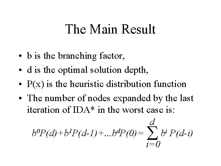
The Main Result • • b is the branching factor, d is the optimal solution depth, P(x) is the heuristic distribution function The number of nodes expanded by the last iteration of IDA* in the worst case is: d b 0 P(d)+b 1 P(d-1)+. . . bd. P(0)= bi P(d-i) i=0

Assumptions of the Analysis • h is consistent, meaning that in any move, h never decreases more than g increases. • The graph is searched as a tree (e. g. IDA*). • Goal nodes are ignored. • The distribution of heuristic values at a given depth approximates the equilibirum heuristic distribution at large depth. • We don’t assume that costs are uniform.

Experiments on Rubik’s Cube • Heuristic function is based on corner cubie and two edge cubie pattern databases. • Heuristic distribution is computed exactly from databases, assuming database values are independent of each other. • Theory predicts average node expansions by IDA* to within 1%.

Experiments on Fifteen Puzzle • Heuristic is Manhattan distance. • Heuristic distribution is approximated by 10 billion random samples of problem space. • Theory predicts average node expansions within 2. 5% at typical solution depths. • Accuracy of theory increases with depth.

Experiments on Eight Puzzle • Heuristic is Manhattan distance. • Heuristic distribution is computed exactly by exhaustive search of entire space. • Average node expansions by IDA* is computed exactly by running every solvable initial state as deep as we need to. • Theory predicts experimental results exactly

Practical Importance • Ability to predict performance of heuristic search from heuristic distribution allows us to choose among alternative heuristics. • More efficient than running large numbers of searches in the problem domain • Can predict performance even if we can’t run any problem instances (e. g. Twenty. Four puzzle with Manhattan distance).

Complexity of Heuristic Search • Complexity of brute-force search is O(bd). • Previous results predicted O((b-K)d) for complexity of heuristic search, reducing the effective branching factor. • Our theory predicts O(bd-k), reducing the effective depth of search by a constant. • This is confirmed by our experiments. • k is roughly the expected value of heuristic.

Summary • More powerful admissible heuristics can be automatically computed by capturing some of the interactions between subproblems. • The time complexity of heuristic search algorithms can be accurately predicted from the branching factor, search depth, and heuristic distribution function.

Conclusions • Recent progress in this area has come from more accurate heuristic functions. • Admissible heuristics can also be used to speed up searches for sub-optimal solutions. • New methods have emerged for constructing such heuristic functions. • Applying these methods to new problems still requires work.