Psychology 242 Introduction to Statistics 2 Revised 111814

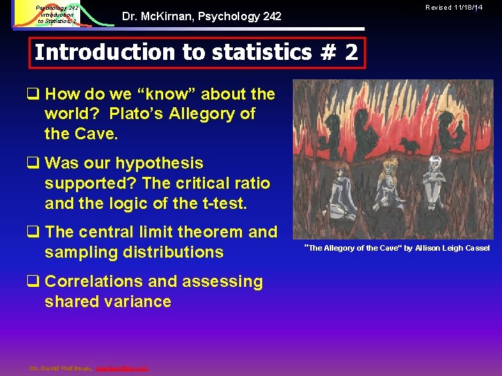
Psychology 242 Introduction to Statistics, 2 Revised 11/18/14 1 Dr. Mc. Kirnan, Psychology 242 Introduction to statistics # 2 q How do we “know” about the world? Plato’s Allegory of the Cave. q Was our hypothesis supported? The critical ratio and the logic of the t-test. q The central limit theorem and sampling distributions q Correlations and assessing shared variance Dr. David Mc. Kirnan, davidmck@uic. edu "The Allegory of the Cave" by Allison Leigh Cassel

2 Psychology 242 Introduction to Statistics, 2 “Earthly knowledge is but shadow” Dr. David Mc. Kirnan, davidmck@uic. edu

Psychology 242 Introduction to Statistics, 2 Plato’s Allegory of the Cave 3 Plato, Republic, Book VII, 514 a-c to 521 a-e) Plato's Allegory of the cave, Engraving of Jan Saenredam (1565 -1607) after a painting of Corneliszoon van Haarlem (1562 -1638) Dr. David Mc. Kirnan, davidmck@uic. edu

Psychology 242 Introduction to Statistics, 2 Plato’s Allegory of the Cave 4 Plato, Republic, Book VII, 514 a-c to 521 a-e) Socrates: And now, I said, let me show in a figure how far our nature is enlightened or unenlightened : "Behold ! , human beings living in a underground den, which has a mouth open towards the light and reaching all along the den. Here they have been from their childhood, and have their legs and necks chained so that they cannot move, and can only see before them, being prevented by the chains from turning round their heads. ” Plato's Allegory of the cave, Engraving of Jan Saenredam (1565 -1607) after a painting of Corneliszoon van Haarlem (1562 -1638) Dr. David Mc. Kirnan, davidmck@uic. edu

Psychology 242 Introduction to Statistics, 2 Plato’s Cave, 2 5 “Above and behind them a fire is blazing at a distance, and between the fire and the prisoners there is a raised way; and you will see, if you look, a low wall built along the way, like the screen which marionette players have in front of them, over which they show the puppets. “ Glaucon: "I see". "And do you see", I said, "men passing along the wall carrying all sorts of vessels, and statues and figures of animals made of wood and stone and various materials, which appear over the wall ? Some of them are talking, others silent. “ Dr. David Mc. Kirnan, davidmck@uic. edu

Psychology 242 Introduction to Statistics, 2 Plato’s Cave, 3 6 Glaucon: "You have shown me a strange image, and they are strange prisoners". "Like ourselves", I replied. "And they see only their own shadows, or the shadows of one another, which the fire throws on the opposite wall of the cave ? " Glaucon: "True", he said. "How could they see anything but the shadows if they were never allowed to move their heads? " Dr. David Mc. Kirnan, davidmck@uic. edu

Psychology 242 Introduction to Statistics, 2 Plato’s Cave, 4 And of the objects which are being carried in like manner they would only see the shadows? " Glaucon: "Yes", he said. "And if they were able to converse with one another, would they not suppose that they were naming what was actually before them? " Glaucon: "Very true. “ Dr. David Mc. Kirnan, davidmck@uic. edu 7

Psychology 242 Introduction to Statistics, 2 Plato’s Cave, 5 "And suppose further that the prison had an echo which came from the other side… would they not be sure to fancy then one of the passersby spoke that the voice which they heard came from the passing shadow ? " Glaucon: "No question", he replied. "To them", I said, "the truth would be literally nothing but the shadows of the images". Glaucon: "That is certain. " Dr. David Mc. Kirnan, davidmck@uic. edu 8

Psychology 242 Introduction to Statistics, 2 9 Plato’s Allegory of the Cave Click here for a link to the full text of Book VII of The Republic by Plato Click the image for a discussion of Plato’s Cave and education in Electrum Magazine. Dr. David Mc. Kirnan, davidmck@uic. edu

Psychology 242 Introduction to Statistics, 2 Plato’s Cave, 6 What does Plato’s Allegory of the Cave tell us about scientific reasoning? We cannot observe “nature” directly, we only see its manifestations or images: ü We are trapped in a world of immediate sensation; ü Our senses routinely deceive us (they have error). ü Only through sustained education can we get outside our limited sensations to see the underlying “form” of nature Dr. David Mc. Kirnan, davidmck@uic. edu 10

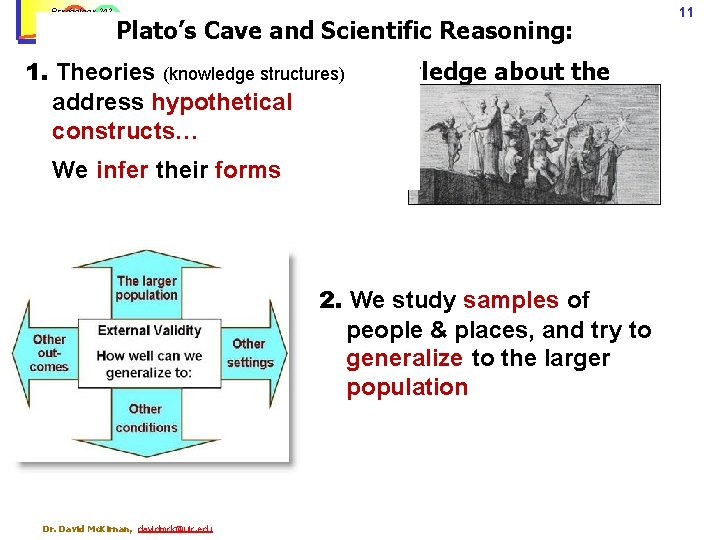
Psychology 242 Introduction to Statistics, 2 Plato’s Cave and Scientific Reasoning: Plato’s Cave, 7 Core limitations of our knowledge about the 1. Theories (knowledge structures) address hypothetical world. constructs… We infer their forms 2. We study samples of people & places, and try to generalize to the larger population Dr. David Mc. Kirnan, davidmck@uic. edu 11

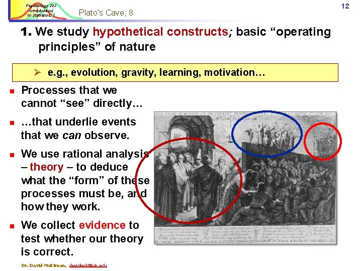
Psychology 242 Introduction to Statistics, 2 Plato’s Cave, 8 1. We study hypothetical constructs; basic “operating principles” of nature Ø e. g. , evolution, gravity, learning, motivation… n n Processes that we cannot “see” directly… …that underlie events that we can observe. We use rational analysis – theory – to deduce what the “form” of these processes must be, and how they work. We collect evidence to test whether our theory is correct. Dr. David Mc. Kirnan, davidmck@uic. edu 12

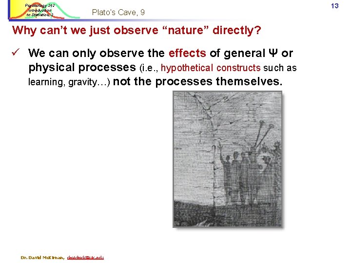
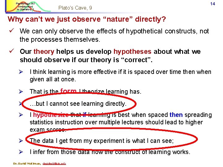
Psychology 242 Introduction to Statistics, 2 Plato’s Cave, 9 Why can’t we just observe “nature” directly? ü We can only observe the effects of general Ψ or physical processes (i. e. , hypothetical constructs such as learning, gravity…) not the processes themselves. Dr. David Mc. Kirnan, davidmck@uic. edu 13

Psychology 242 Introduction to Statistics, 2 Plato’s Cave, 9 14 Why can’t we just observe “nature” directly? ü We can only observe the effects of hypothetical constructs, not the processes themselves. ü Our theory helps us develop hypotheses about what we should observe if our theory is “correct”. Ø I think learning is more effective if it is spaced over time then when given all at once. Ø That is the form I theorize learning has. Ø …but I cannot see learning directly. Ø I hypothesize that if learning is best when spaced then spreading statistics instruction over multiple lectures should lead to higher exam scores. Ø The data I get from my experiment is what I can see; Ø I infer from those data how the construct of learning works. Dr. David Mc. Kirnan, davidmck@uic. edu

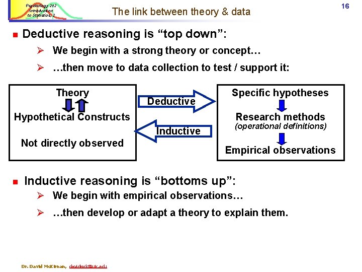
Psychology 242 Introduction to Statistics, 2 Plato’s Cave, 9 15 Why can’t we just observe “nature” directly? ü We can only observe the effects of hypothetical constructs, not the processes themselves. ü Our theory helps us develop hypotheses about what we should observe if our theory is “correct”. ü We test our hypotheses to infer how nature works. ü Our inferences contain error: we must estimate the probability that our results are due to “real” effects versus chance. ü The link from hypothetical constructs to empirical evidence can be deductive (“top-down”) or inductive (“bottoms-up”). Dr. David Mc. Kirnan, davidmck@uic. edu

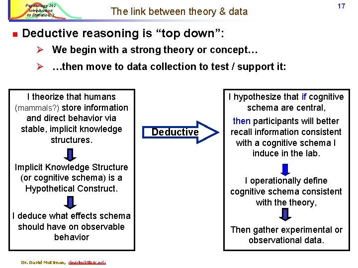
Psychology 242 Introduction to Statistics, 2 n The link between theory & data Deductive reasoning is “top down”: Ø We begin with a strong theory or concept… Ø …then move to data collection to test / support it: Theory Deductive Hypothetical Constructs Research methods Inductive Not directly observed n Specific hypotheses (operational definitions) Empirical observations Inductive reasoning is “bottoms up”: Ø We begin with empirical observations… Ø …then develop or adapt a theory to explain them. Dr. David Mc. Kirnan, davidmck@uic. edu 16

Psychology 242 Introduction to Statistics, 2 n The link between theory & data 17 Deductive reasoning is “top down”: Ø We begin with a strong theory or concept… Ø …then move to data collection to test / support it: I theorize that humans (mammals? ) store information and direct behavior via stable, implicit knowledge structures. Implicit Knowledge Structure (or cognitive schema) is a Hypothetical Construct. I deduce what effects schema should have on observable behavior Dr. David Mc. Kirnan, davidmck@uic. edu I hypothesize that if cognitive schema are central, Deductive then participants will better recall information consistent with a cognitive schema I induce in the lab. I operationally define cognitive schema consistent with theory, Then gather experimental or observational data.

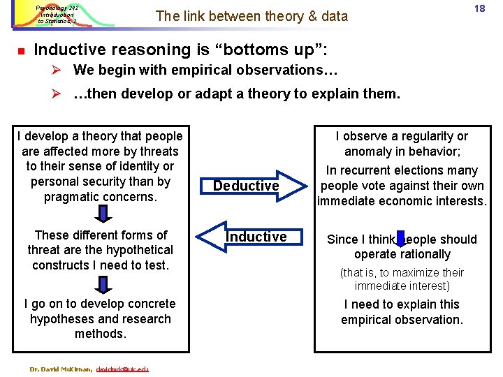
Psychology 242 Introduction to Statistics, 2 n The link between theory & data 18 Inductive reasoning is “bottoms up”: Ø We begin with empirical observations… Ø …then develop or adapt a theory to explain them. I develop a theory that people are affected more by threats to their sense of identity or personal security than by pragmatic concerns. These different forms of threat are the hypothetical constructs I need to test. I go on to develop concrete hypotheses and research methods. Dr. David Mc. Kirnan, davidmck@uic. edu I observe a regularity or anomaly in behavior; Deductive In recurrent elections many people vote against their own immediate economic interests. Since I think people should operate rationally (that is, to maximize their immediate interest) I need to explain this empirical observation.

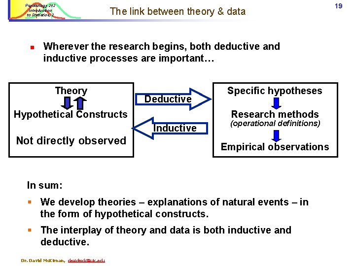
Psychology 242 Introduction to Statistics, 2 n The link between theory & data Wherever the research begins, both deductive and inductive processes are important… Theory Deductive Hypothetical Constructs Research methods Inductive Not directly observed Specific hypotheses (operational definitions) Empirical observations In sum: § We develop theories – explanations of natural events – in the form of hypothetical constructs. § The interplay of theory and data is both inductive and deductive. Dr. David Mc. Kirnan, davidmck@uic. edu 19

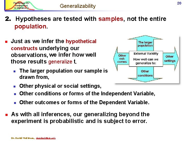
Psychology 242 Introduction to Statistics, 2 Generalizability 2. Hypotheses are tested with samples, not the entire population. n Just as we infer the hypothetical constructs underlying our observations, we infer how well those results generalize to: . n n Other physical or social settings, Other conditions or forms of the Independent Variable, n Other outcomes or forms of the Dependent Variable. n n The larger population our sample is drawn from, As with all inferences, our generalizing beyond the experiment is probabilistic and is subject to error. David Mc. Kirnan, davidmck@uic. edu 20

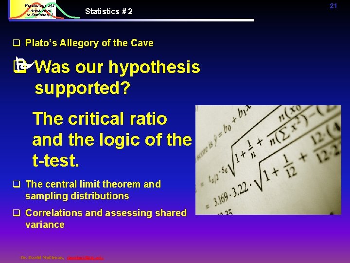
Psychology 242 Introduction to Statistics, 2 Statistics # 2 q Plato’s Allegory of the Cave Was our hypothesis q supported? The critical ratio and the logic of the t-test. q The central limit theorem and sampling distributions q Correlations and assessing shared variance Dr. David Mc. Kirnan, davidmck@uic. edu 21

Psychology 242 Introduction to Statistics, 2 Using statistics to test hypotheses: Core concept: ü No scientific finding is “absolutely” true. ü Any effect is probabilistic: Ø Ø We use empirical data to infer how the world words. Our inferences are subject to error: The outcome we think we see may not be ‘real’. We judge whether our inference is justified by how likely it would be for the outcome to occur by chance alone. We use the normal distribution to help us determine how likely an research outcome would be by chance alone Dr. David Mc. Kirnan, davidmck@uic. edu 22

Psychology 242 Introduction to Statistics, 2 Probabilities & Statistical Hypothesis Testing 23 Null Hypothesis: All scores differ from the M by chance alone. Scientific observations are “innocent until proven guilty”. For any research outcome: ü Testing how far a score is from the mean, ü Comparing two groups, ü Testing whether two variables are correlated. The odds of the outcome occurring by chance alone is always greater than 0. We cannot just take any result and call it meaningful, since any result may be due to chance, not the Independent Variable. So, we assume any result is by chance unless it is so strong that it is unlikely to occur randomly. Dr. David Mc. Kirnan, davidmck@uic. edu

Psychology 242 Introduction to Statistics, 2 Probabilities & Statistical Hypothesis Testing Null Hypothesis: All scores differ from the M by chance alone. Alternate (experimental) hypothesis: This score is extreme enough (these results are strong enough…) that is it unlikely to have occurred by chance alone. Using the Normal Distribution: n n n More extreme scores have a lower probability of occurring by chance alone Z = the % of cases above or below the observed score A high Z score may be “extreme” enough for us to reject the null hypothesis Dr. David Mc. Kirnan, davidmck@uic. edu 24

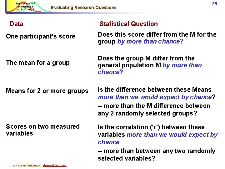
Psychology 242 Introduction to Statistics, 2 Evaluating Research Questions Data 25 Statistical Question One participant’s score Does this score differ from the M for the group by more than chance? The mean for a group Does the group M differ from the general population M by more than chance? Means for 2 or more groups Is the difference between these Means more than we would expect by chance? -- more than the M difference between any 2 randomly selected groups? Scores on two measured variables Is the correlation (‘r’) between these variables more than we would expect by chance -- more than between any two randomly selected variables? Dr. David Mc. Kirnan, davidmck@uic. edu

Psychology 242 Introduction to Statistics, 2 Critical ratio We answer our “more than we would expect by chance” question using the Critical Ratio. Dr. David Mc. Kirnan, davidmck@uic. edu 26

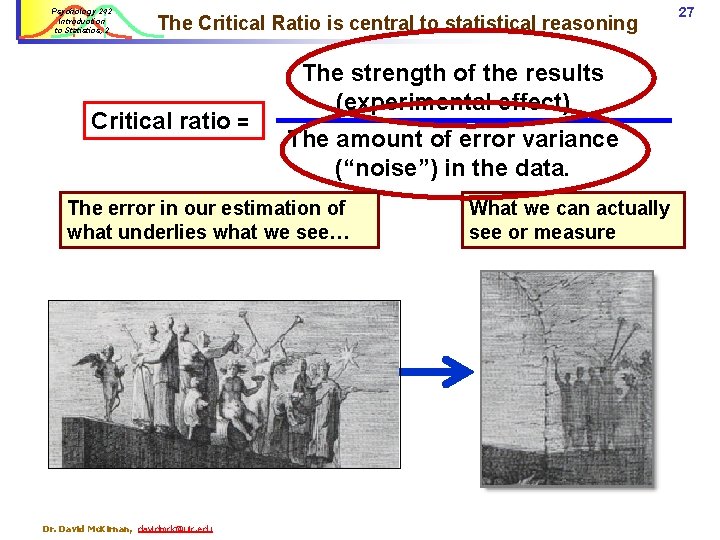
Psychology 242 Introduction to Statistics, 2 The Critical Ratio is central to statistical reasoning Critical ratio = The strength of the results (experimental effect) The amount of error variance (“noise”) in the data. The error in our estimation of what underlies what we see… Dr. David Mc. Kirnan, davidmck@uic. edu What we can actually see or measure 27

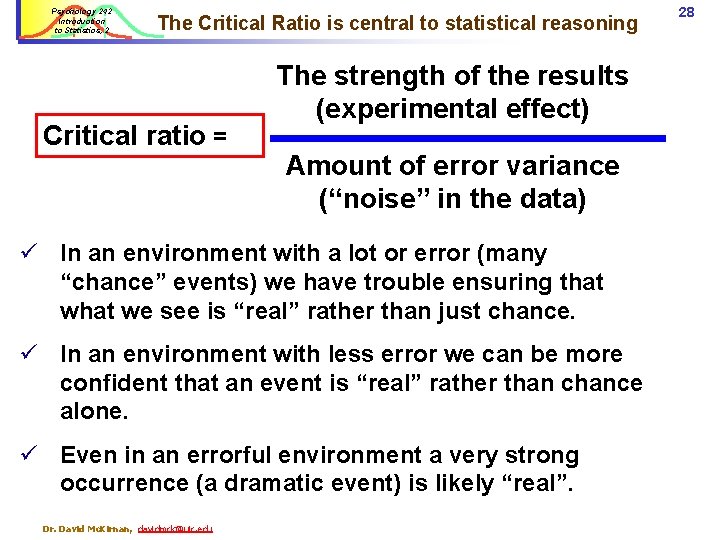
Psychology 242 Introduction to Statistics, 2 The Critical Ratio is central to statistical reasoning Critical ratio = The strength of the results (experimental effect) Amount of error variance (“noise” in the data) ü In an environment with a lot or error (many “chance” events) we have trouble ensuring that we see is “real” rather than just chance. ü In an environment with less error we can be more confident that an event is “real” rather than chance alone. ü Even in an errorful environment a very strong occurrence (a dramatic event) is likely “real”. Dr. David Mc. Kirnan, davidmck@uic. edu 28

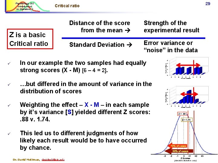
Psychology 242 Introduction to Statistics, 2 Z is a basic Critical ratio ü ü 29 Critical ratio Distance of the score from the mean Strength of the experimental result Standard Deviation Error variance or “noise” in the data In our example the two samples had equally strong scores (X - M) [6 – 4 = 2]. …but differed in the amount of variance in the distribution of scores Weighting the effect – X - M – in each sample by it’s variance [S] yielded different Z scores: . 88 v. 1. 74. This led us to different judgments of how likely each result would be to have occurred by chance. Dr. David Mc. Kirnan, davidmck@uic. edu

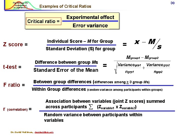
Psychology 242 Introduction to Statistics, 2 Z score = t-test = F ratio = r (correlation) = 30 Examples of Critical Ratios Individual Score – M for Group Standard Deviation (S) for group Difference between group Ms Standard Error of the Mean = = Between group differences (differences among > 3 group Ms) Within Group differences (random variance among participants within groups) Association between variables (joint Z scores) summed across participants (Zvariable 1 x Zvariable 2) Random variance between participants within variables Dr. David Mc. Kirnan, davidmck@uic. edu

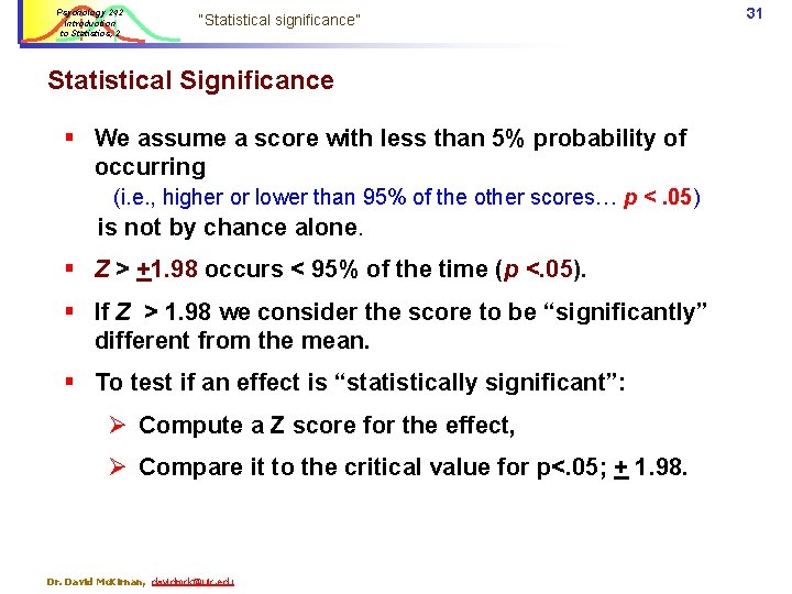
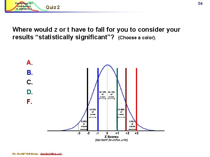
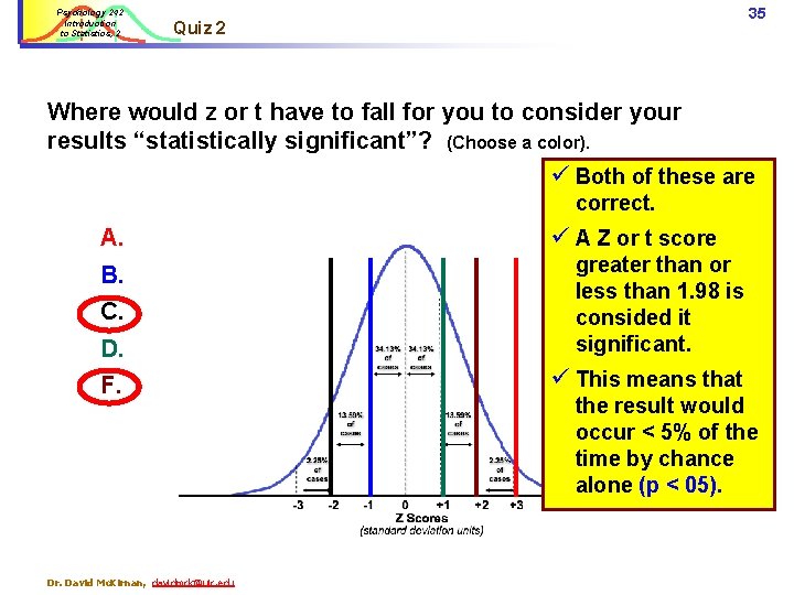
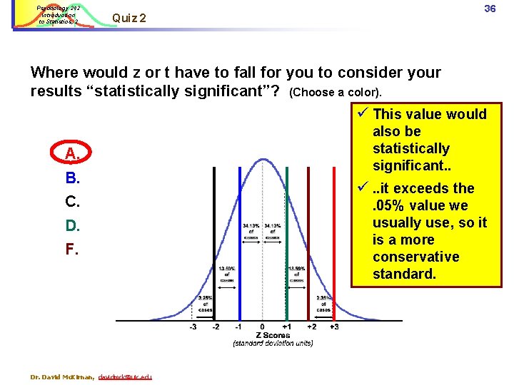
Psychology 242 Introduction to Statistics, 2 “Statistical significance” Statistical Significance § We assume a score with less than 5% probability of occurring (i. e. , higher or lower than 95% of the other scores… p <. 05) is not by chance alone. § Z > +1. 98 occurs < 95% of the time (p <. 05). § If Z > 1. 98 we consider the score to be “significantly” different from the mean. § To test if an effect is “statistically significant”: Ø Compute a Z score for the effect, Ø Compare it to the critical value for p<. 05; + 1. 98. Dr. David Mc. Kirnan, davidmck@uic. edu 31

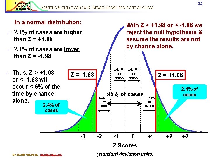
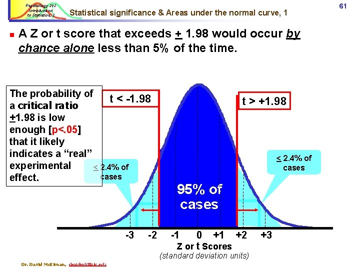
Psychology 242 Introduction to Statistics, 2 In a normal distribution: ü ü ü 32 Statistical significance & Areas under the normal curve With Z > +1. 98 or < -1. 98 we reject the null hypothesis & assume the results are not by chance alone. 2. 4% of cases are higher than Z = +1. 98 2. 4% of cases are lower than Z = -1. 98 Thus, Z > +1. 98 or < -1. 98 will occur < 5% of the time by chance alone. 34. 13% of of cases Z = -1. 98 Z = +1. 98 95% of cases 13. 59% of cases 2. 4% of cases 2. 25% of cases -3 2. 25% of cases -2 -1 0 +1 Z Scores Dr. David Mc. Kirnan, davidmck@uic. edu 2. 4% of cases (standard deviation units) +2 +3

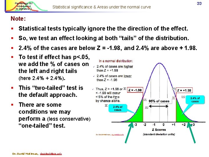
Psychology 242 Introduction to Statistics, 2 Statistical significance & Areas under the normal curve 33 Note: § Statistical tests typically ignore the direction of the effect. § So, we test an effect looking at both “tails” of the distribution. § 2. 4% of the cases are below Z = -1. 98, and 2. 4% are above + 1. 98. § To test if effect has p<. 05, we add the % of cases on the left and right tails (here 2. 4% + 2. 4%). § This “two-tailed” test is the default approach. § There are some conditions we may perform a (less conservative) “one-tailed” test. Dr. David Mc. Kirnan, davidmck@uic. edu

Psychology 242 Introduction to Statistics, 2 Quiz 2 Where would z or t have to fall for you to consider your results “statistically significant”? (Choose a color). A. B. C. D. F. Dr. David Mc. Kirnan, davidmck@uic. edu 34

Psychology 242 Introduction to Statistics, 2 35 Quiz 2 Where would z or t have to fall for you to consider your results “statistically significant”? (Choose a color). ü Both of these are correct. A. ü A Z or t score D. greater than or less than 1. 98 is consided it significant. F. ü This means that B. C. Dr. David Mc. Kirnan, davidmck@uic. edu the result would occur < 5% of the time by chance alone (p < 05).

Psychology 242 Introduction to Statistics, 2 36 Quiz 2 Where would z or t have to fall for you to consider your results “statistically significant”? (Choose a color). ü This value would A. B. C. D. F. Dr. David Mc. Kirnan, davidmck@uic. edu also be statistically significant. . ü. . it exceeds the. 05% value we usually use, so it is a more conservative standard.

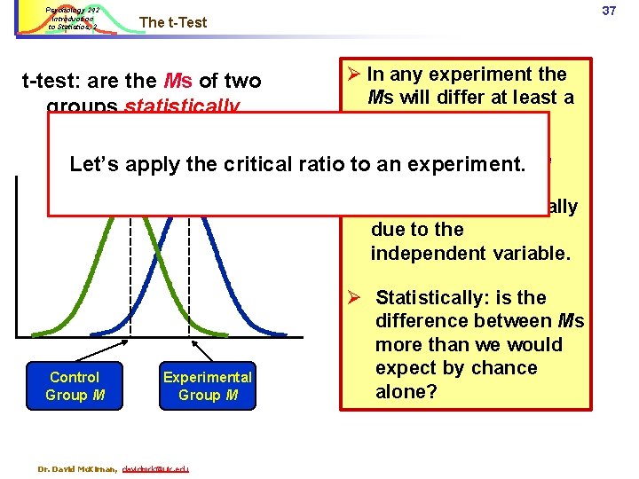
Psychology 242 Introduction to Statistics, 2 37 The t-Test t-test: are the Ms of two groups statistically different from each other? Ø In any experiment the Ms will differ at least a little. the difference Let’s apply the critical ratio Ø to. Does an experiment. we observe reflect “reality”? … i. e. , really due to the independent variable. Control Group M Experimental Group M Dr. David Mc. Kirnan, davidmck@uic. edu Ø Statistically: is the difference between Ms more than we would expect by chance alone?

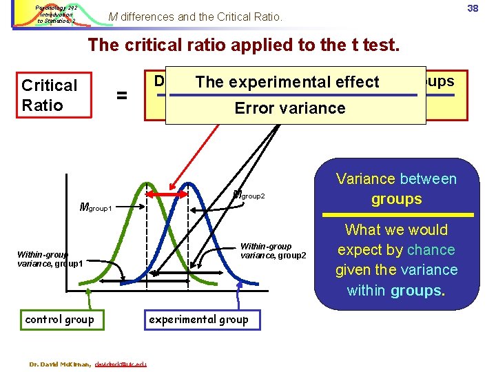
Psychology 242 Introduction to Statistics, 2 38 M differences and the Critical Ratio. The critical ratio applied to the t test. Critical Ratio = Difference between Ms foreffect the two groups The experimental Variability groups (error) Errorwithin variance Mgroup 2 Mgroup 1 Within-group variance, group 1 control group Dr. David Mc. Kirnan, davidmck@uic. edu Within-group variance, group 2 experimental group Variance between groups What we would expect by chance given the variance within groups.

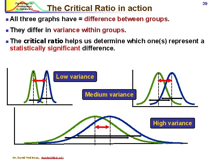
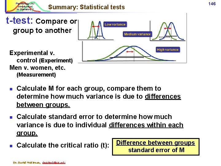
Psychology 242 Introduction to Statistics, 2 39 The Critical Ratio in action n All three graphs have = difference between groups. n They differ in variance within groups. n The critical ratio helps us determine which one(s) represent a statistically significant difference. Low variance Medium variance High variance Dr. David Mc. Kirnan, davidmck@uic. edu

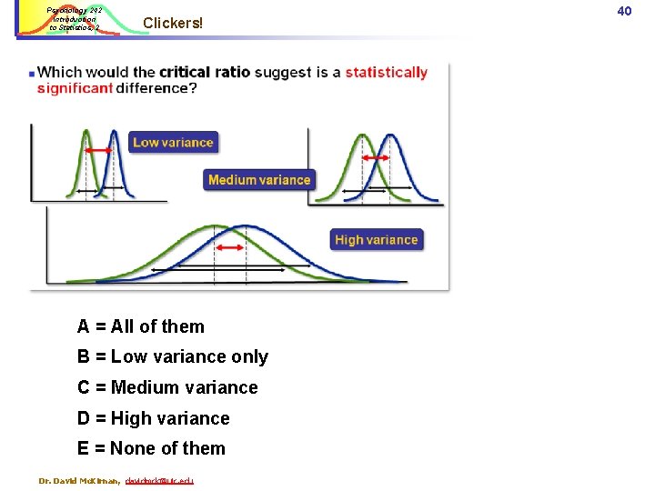
Psychology 242 Introduction to Statistics, 2 Clickers! A = All of them B = Low variance only C = Medium variance D = High variance E = None of them Dr. David Mc. Kirnan, davidmck@uic. edu 40

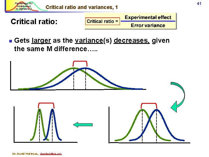
Psychology 242 Introduction to Statistics, 2 Critical ratio and variances, 1 Critical ratio: n Gets larger as the variance(s) decreases, given the same M difference…. . Dr. David Mc. Kirnan, davidmck@uic. edu 41

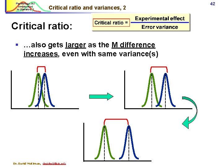
Psychology 242 Introduction to Statistics, 2 Critical ratio and variances, 2 Critical ratio: § …also gets larger as the M difference increases, even with same variance(s) Dr. David Mc. Kirnan, davidmck@uic. edu 42

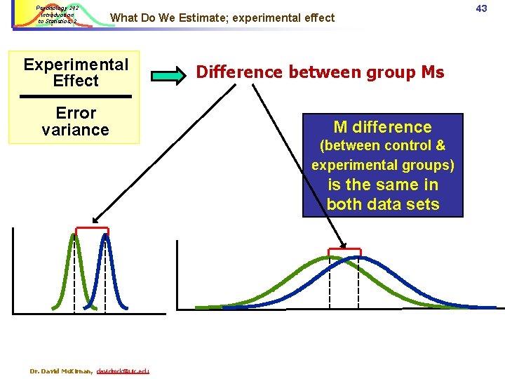
Psychology 242 Introduction to Statistics, 2 What Do We Estimate; experimental effect Experimental Effect Error variance Difference between group Ms M difference (between control & experimental groups) is the same in both data sets Dr. David Mc. Kirnan, davidmck@uic. edu 43

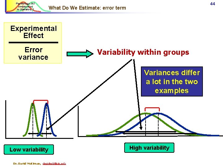
Psychology 242 Introduction to Statistics, 2 44 What Do We Estimate: error term Experimental Effect Error variance Variability within groups Variances differ a lot in the two examples Low variability Dr. David Mc. Kirnan, davidmck@uic. edu High variability

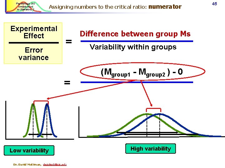
Psychology 242 Introduction to Statistics, 2 Assigning numbers to the critical ratio: Experimental Effect Error variance = = Low variability Dr. David Mc. Kirnan, davidmck@uic. edu numerator Difference between group Ms Variability within groups (Mgroup 1 - Mgroup 2 ) - 0 High variability 45

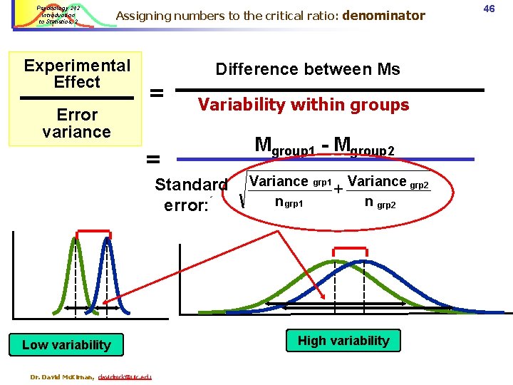
Psychology 242 Introduction to Statistics, 2 Assigning numbers to the critical ratio: denominator Experimental Effect Error variance Difference between Ms = Variability within groups = Standard error: Low variability Dr. David Mc. Kirnan, davidmck@uic. edu Mgroup 1 - Mgroup 2 Variance n grp 1 + Variance grp 2 n grp 2 High variability 46

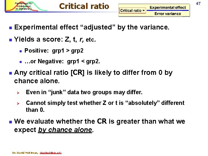
Psychology 242 Introduction to Statistics, 2 Critical ratio n Experimental effect “adjusted” by the variance. n Yields a score: Z, t, r, etc. n n Positive: grp 1 > grp 2 n …or Negative: grp 1 < grp 2. Any critical ratio [CR] is likely to differ from 0 by chance alone. Ø Ø n Even in “junk” data two groups may differ. Cannot simply test whether Z or t is “absolutely” different than 0. We evaluate whether the CR is greater than what we expect by chance alone. Dr. David Mc. Kirnan, davidmck@uic. edu 47

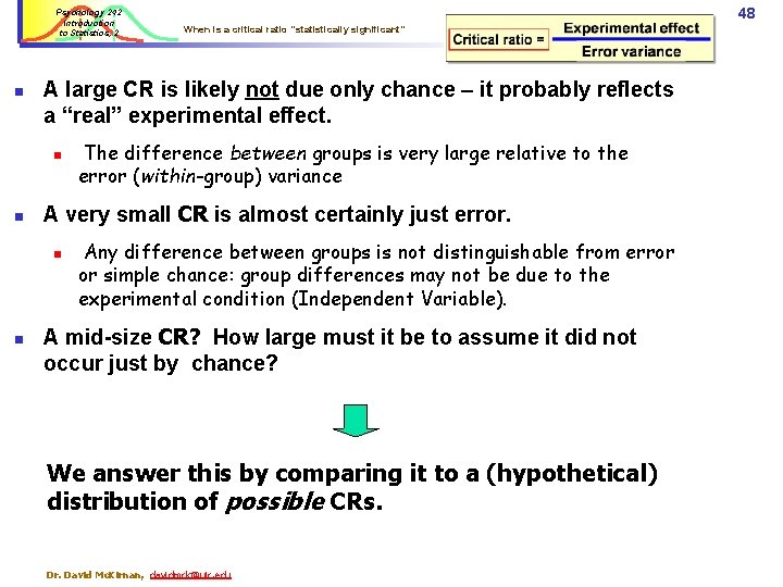
Psychology 242 Introduction to Statistics, 2 n A large CR is likely not due only chance – it probably reflects a “real” experimental effect. n n The difference between groups is very large relative to the error (within-group) variance A very small CR is almost certainly just error. n n 48 When is a critical ratio “statistically significant” Any difference between groups is not distinguishable from error or simple chance: group differences may not be due to the experimental condition (Independent Variable). A mid-size CR? How large must it be to assume it did not occur just by chance? We answer this by comparing it to a (hypothetical) distribution of possible CRs. Dr. David Mc. Kirnan, davidmck@uic. edu

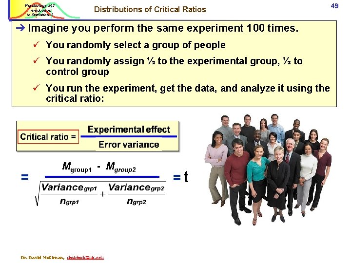
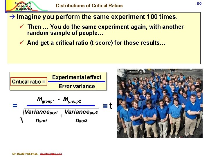
Psychology 242 Introduction to Statistics, 2 Distributions of Critical Ratios ➔ Imagine you perform the same experiment 100 times. ü You randomly select a group of people ü You randomly assign ½ to the experimental group, ½ to control group ü You run the experiment, get the data, and analyze it using the critical ratio: = Mgroup 1 - Mgroup 2 Dr. David Mc. Kirnan, davidmck@uic. edu =t 49

Psychology 242 Introduction to Statistics, 2 Distributions of Critical Ratios ➔ Imagine you perform the same experiment 100 times. ü Then … You do the same experiment again, with another random sample of people… ü And get a critical ratio (t score) for those results… = Mgroup 1 - Mgroup 2 Dr. David Mc. Kirnan, davidmck@uic. edu =t 50

Psychology 242 Introduction to Statistics, 2 Distributions of Critical Ratios ➔ Imagine you perform the same experiment 100 times. ü And you get yet another sample… ü And get a critical ratio (t score) for those results… = Mgroup 1 - Mgroup 2 Dr. David Mc. Kirnan, davidmck@uic. edu =t 51

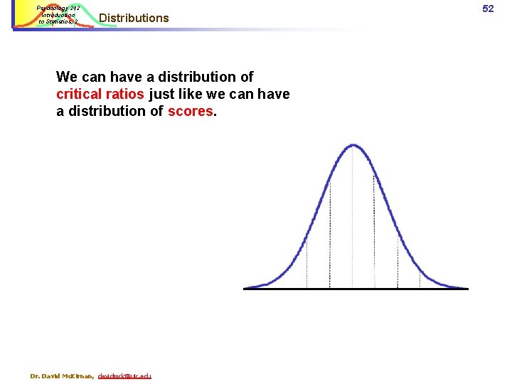
Psychology 242 Introduction to Statistics, 2 Distributions We can have a distribution of critical ratios just like we can have a distribution of scores. Dr. David Mc. Kirnan, davidmck@uic. edu 52

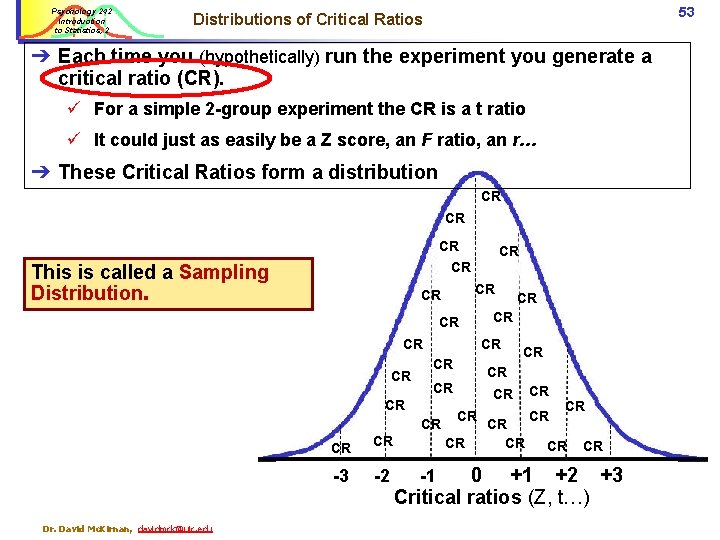
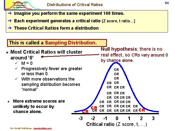
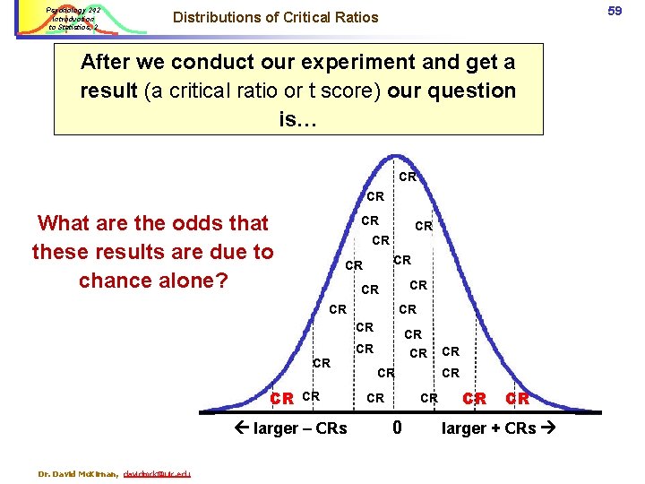
Psychology 242 Introduction to Statistics, 2 53 Distributions of Critical Ratios ➔ Each time you (hypothetically) run the experiment you generate a critical ratio (CR). ü For a simple 2 -group experiment the CR is a t ratio ü It could just as easily be a Z score, an F ratio, an r… ➔ These Critical Ratios form a distribution CR CR CR This is called a Sampling Distribution. CR CR CR -3 Dr. David Mc. Kirnan, davidmck@uic. edu CR -2 CR CR CR CR CR 0 +1 +2 +3 Critical ratios (Z, t…) -1

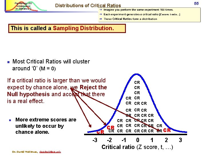
Psychology 242 Introduction to Statistics, 2 54 Distributions of Critical Ratios ➔ Imagine you perform the same experiment 100 times. ➔ Each experiment generates a critical ratio [Z score, t ratio…] ➔ These Critical Ratios form a distribution This is called a Sampling Distribution. n Null hypothesis; there is no real effect, so CRs vary around 0 Most Critical Ratios will cluster around ‘ 0’ by chance alone. ü M=0 ü Progressively fewer are greater or less than 0. ü With more observations the sampling distribution becomes “normal” n More extreme scores are unlikely to occur by chance alone. CR -3 Dr. David Mc. Kirnan, davidmck@uic. edu CR CR CR CR CR CR CR CR CR -2 -1 0 1 2 Critical ratio (Z score, t, …) 3

Psychology 242 Introduction to Statistics, 2 55 Distributions of Critical Ratios This is called a Sampling Distribution. n Most Critical Ratios will cluster around ‘ 0’ (M = 0) If a critical ratio is larger than we would expect by chance alone, we Reject the Null hypothesis and accept that there is a real effect. n More extreme scores are unlikely to occur by chance alone. CR -3 Dr. David Mc. Kirnan, davidmck@uic. edu CR CR CR CR CR CR CR CR CR -2 -1 0 1 2 Critical ratio (Z score, t, …) 3

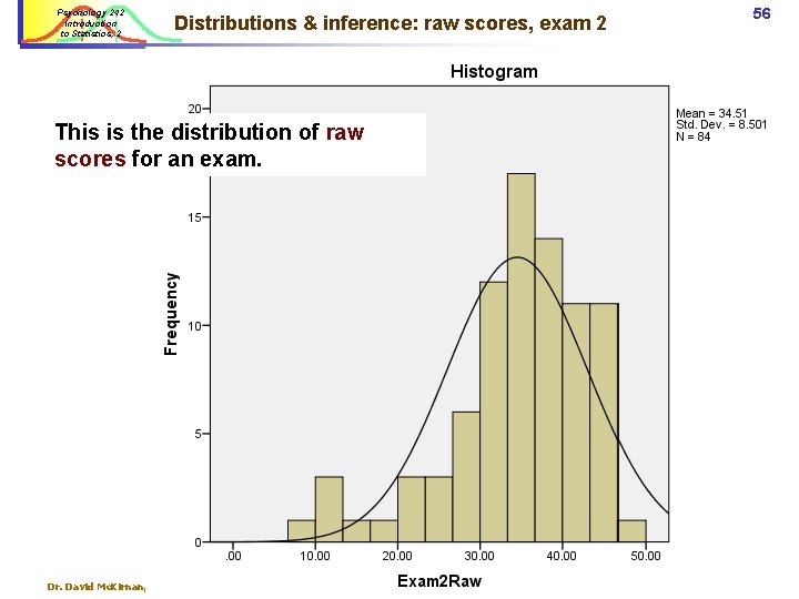
Psychology 242 Introduction to Statistics, 2 Distributions & inference: raw scores, exam 2 This is the distribution of raw scores for an exam. Dr. David Mc. Kirnan, davidmck@uic. edu Statistics Introduction 2. 56

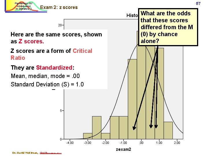
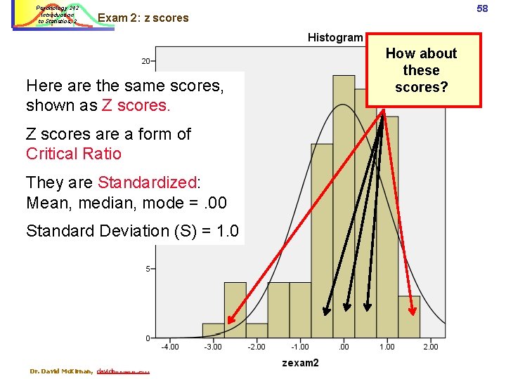
Psychology 242 Introduction to Statistics, 2 57 Exam 2: z scores Here are the same scores, shown as Z scores. What are the odds that these scores differed from the M (0) by chance alone? Z scores are a form of Critical Ratio They are Standardized: Mean, median, mode =. 00 Standard Deviation (S) = 1. 0 Dr. David Mc. Kirnan, davidmck@uic. edu Statistics Introduction 2.

Psychology 242 Introduction to Statistics, 2 58 Exam 2: z scores Here are the same scores, shown as Z scores are a form of Critical Ratio They are Standardized: Mean, median, mode =. 00 Standard Deviation (S) = 1. 0 Dr. David Mc. Kirnan, davidmck@uic. edu How about these scores?

Psychology 242 Introduction to Statistics, 2 59 Distributions of Critical Ratios After we conduct our experiment and get a result (a critical ratio or t score) our question is… CR CR What are the odds that these results are due to chance alone? CR CR CR CR larger – CRs Dr. David Mc. Kirnan, davidmck@uic. edu CR CR CR 0 CR CR CR larger + CRs

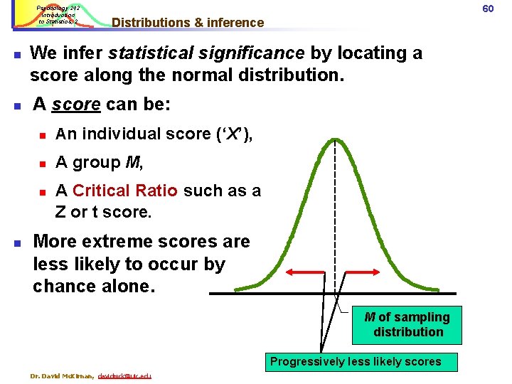
Psychology 242 Introduction to Statistics, 2 n n Distributions & inference We infer statistical significance by locating a score along the normal distribution. A score can be: n An individual score (‘X’), n A group M, n n 60 A Critical Ratio such as a Z or t score. More extreme scores are less likely to occur by chance alone. M of sampling distribution Progressively less likely scores Dr. David Mc. Kirnan, davidmck@uic. edu

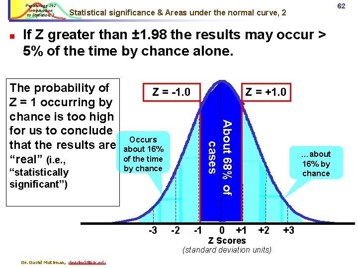
Psychology 242 Introduction to Statistics, 2 n Statistical significance & Areas under the normal curve, 1 A Z or t score that exceeds + 1. 98 would occur by chance alone less than 5% of the time. The probability of t < -1. 98 a critical ratio +1. 98 is low enough [p<. 05] that it likely indicates a “real” experimental < 2. 4% of cases effect. -3 -2 t > +1. 98 < 2. 4% of cases 95% of cases -1 0 +1 +2 Z or t Scores (standard deviation units) Dr. David Mc. Kirnan, davidmck@uic. edu +3 61

Psychology 242 Introduction to Statistics, 2 n 62 Statistical significance & Areas under the normal curve, 2 If Z greater than ± 1. 98 the results may occur > 5% of the time by chance alone. “statistically significant”) Z = -1. 0 Z = +1. 0 About 68% of cases The probability of Z = 1 occurring by chance is too high for us to conclude that the results are “real” (i. e. , Occurs about 16% of the time by chance -3 -2 -1 0 …about 16% by chance +1 Z Scores +2 (standard deviation units) Dr. David Mc. Kirnan, davidmck@uic. edu +3

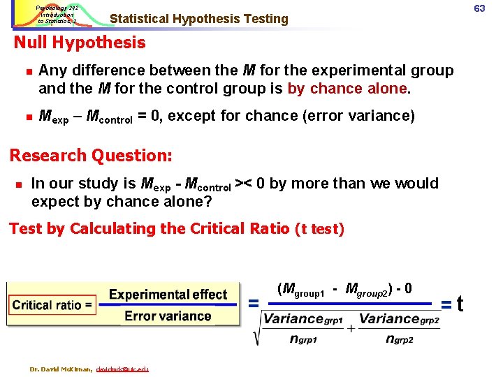
Psychology 242 Introduction to Statistics, 2 63 Statistical Hypothesis Testing Null Hypothesis n n Any difference between the M for the experimental group and the M for the control group is by chance alone. Mexp – Mcontrol = 0, except for chance (error variance) Research Question: n In our study is Mexp - Mcontrol >< 0 by more than we would expect by chance alone? Test by Calculating the Critical Ratio (t test) = Dr. David Mc. Kirnan, davidmck@uic. edu (Mgroup 1 - Mgroup 2) - 0 =t

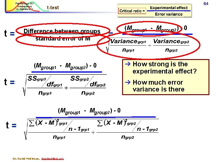
Psychology 242 Introduction to Statistics, 2 t= 64 t-test Difference between groups standard error of M = (Mgroup 1 - Mgroup 2) - 0 t= (Mgroup 1 - Mgroup 2) - 0 ➔ How strong is the experimental effect? ➔ How much error variance is there (Mgroup 1 - Mgroup 2) - 0 t= Dr. David Mc. Kirnan, davidmck@uic. edu

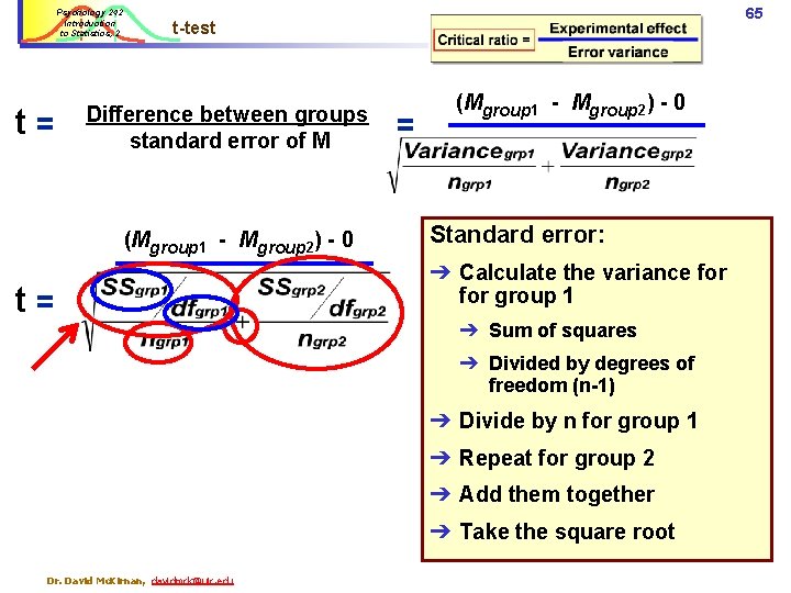
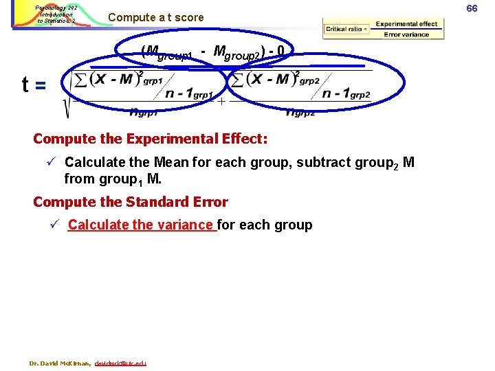
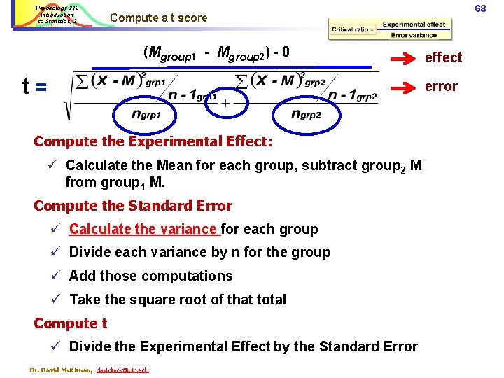
Psychology 242 Introduction to Statistics, 2 t= 65 t-test Difference between groups standard error of M (Mgroup 1 - Mgroup 2) - 0 t= = (Mgroup 1 - Mgroup 2) - 0 Standard error: ➔ Calculate the variance for group 1 ➔ Sum of squares ➔ Divided by degrees of freedom (n-1) ➔ Divide by n for group 1 ➔ Repeat for group 2 ➔ Add them together ➔ Take the square root Dr. David Mc. Kirnan, davidmck@uic. edu

Psychology 242 Introduction to Statistics, 2 Compute a t score (Mgroup 1 - Mgroup 2) - 0 t= Compute the Experimental Effect: ü Calculate the Mean for each group, subtract group 2 M from group 1 M. Compute the Standard Error ü Calculate the variance for each group Dr. David Mc. Kirnan, davidmck@uic. edu 66

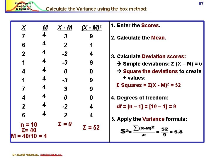
67 Psychology 242 Introduction to Statistics, 2 Calculate the Variance using the box method: X 7 M 4 X-M 3 (X - M)2 9 6 2 1 4 1 7 4 4 4 4 4 2 -2 -3 0 -3 3 4 4 9 0 9 9 0 -2 2 Σ=0 0 4 4 4 2 6 n = 10 Σ= 40 M = 40/10 = 4 Dr. David Mc. Kirnan, davidmck@uic. edu Σ = 52 1. Enter the Scores. 2. Calculate the Mean. 3. Calculate Deviation scores: Simple deviations: Σ (X – M) = 0 Square the deviations to create + values: Σ Squares = Σ(X - M)2 = 52 4. Degrees of freedom: df = [n – 1] = [10 – 1] = 9 5. Apply the Variance formula:

Psychology 242 Introduction to Statistics, 2 68 Compute a t score (Mgroup 1 - Mgroup 2) - 0 t= effect error Compute the Experimental Effect: ü Calculate the Mean for each group, subtract group 2 M from group 1 M. Compute the Standard Error ü Calculate the variance for each group ü Divide each variance by n for the group ü Add those computations ü Take the square root of that total Compute t ü Divide the Experimental Effect by the Standard Error Dr. David Mc. Kirnan, davidmck@uic. edu

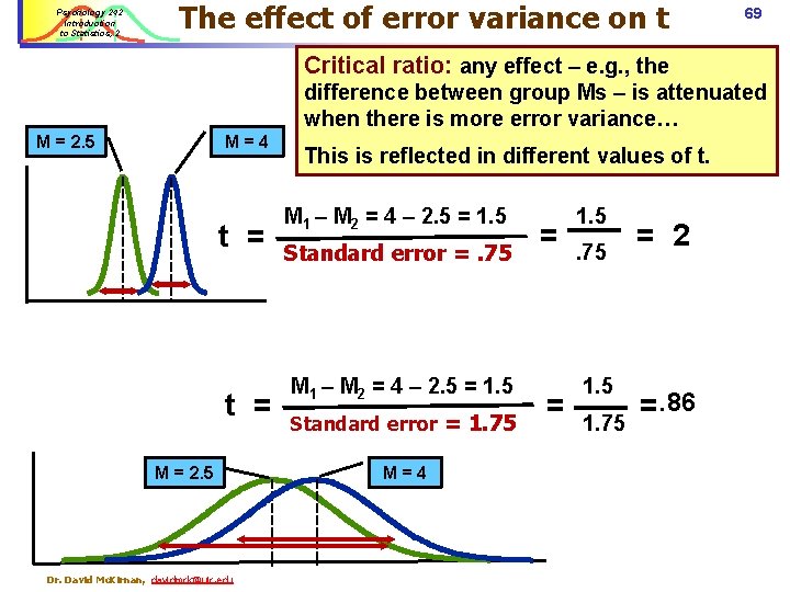
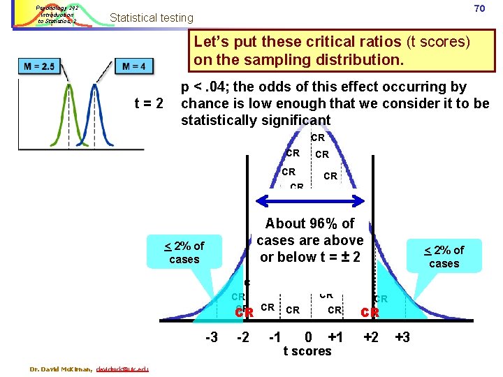
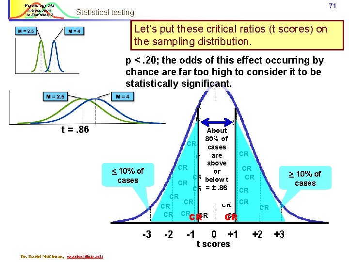
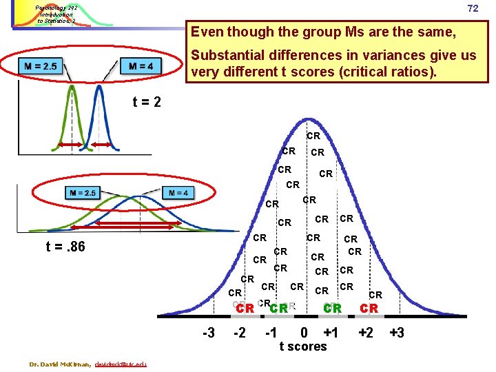
Psychology 242 Introduction to Statistics, 2 The effect of error variance on t 69 Critical ratio: any effect – e. g. , the difference between group Ms – is attenuated when there is more error variance… M = 2. 5 M=4 t = M = 2. 5 Dr. David Mc. Kirnan, davidmck@uic. edu This is reflected in different values of t. M 1 – M 2 = 4 – 2. 5 = 1. 5 Standard error =. 75 M 1 – M 2 = 4 – 2. 5 = 1. 5 Standard error = 1. 75 M=4 = = 1. 5. 75 1. 75 = 2 =. 86

Psychology 242 Introduction to Statistics, 2 70 Statistical testing Let’s put these critical ratios (t scores) on the sampling distribution. t=2 p <. 04; the odds of this effect occurring by chance is low enough that we consider it to be statistically significant CR CR CR of About CR 96% CR CRabove cases are CR CR CR or below t=± 2 CR CR < 2% of cases CR CR CR -3 Dr. David Mc. Kirnan, davidmck@uic. edu -2 -1 0 CR CR < 2% of cases CR CR CR +1 +2 t scores +3

Psychology 242 Introduction to Statistics, 2 71 Statistical testing Let’s put these critical ratios (t scores) on the sampling distribution. p <. 20; the odds of this effect occurring by chance are far too high to consider it to be statistically significant. CR CR CR t =. 86 < 10% of cases -3 Dr. David Mc. Kirnan, davidmck@uic. edu CR CR About 80% CRof CR cases CR are. CR CR above CR CR CR or CR below t CR CR = ±. 86 CR CR CR CR -2 -1 0 +1 t scores +2 > 10% of cases +3

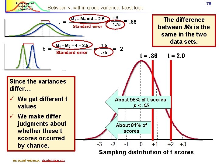
72 Psychology 242 Introduction to Statistics, 2 Even though the group Ms are the same, Substantial differences in variances give us very different t scores (critical ratios). t=2 CR CR CR t =. 86 CR CR CR Dr. David Mc. Kirnan, davidmck@uic. edu -2 CR -1 CR CR CRCR CR CR -3 CR 0 CR CR +1 +2 t scores +3

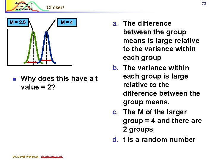
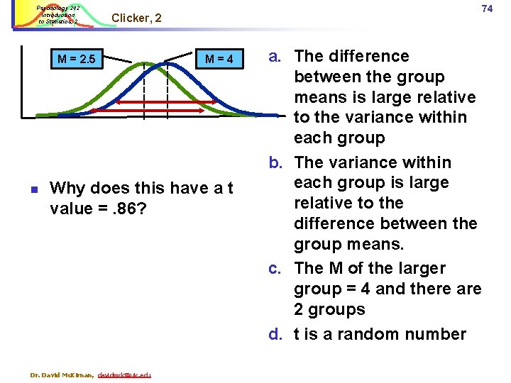
Psychology 242 Introduction to Statistics, 2 M = 2. 5 n Clicker! M=4 Why does this have a t value = 2? Dr. David Mc. Kirnan, davidmck@uic. edu 73 a. The difference between the group means is large relative to the variance within each group b. The variance within each group is large relative to the difference between the group means. c. The M of the larger group = 4 and there are 2 groups d. t is a random number

Psychology 242 Introduction to Statistics, 2 M = 2. 5 n 74 Clicker, 2 M=4 Why does this have a t value =. 86? Dr. David Mc. Kirnan, davidmck@uic. edu a. The difference between the group means is large relative to the variance within each group b. The variance within each group is large relative to the difference between the group means. c. The M of the larger group = 4 and there are 2 groups d. t is a random number

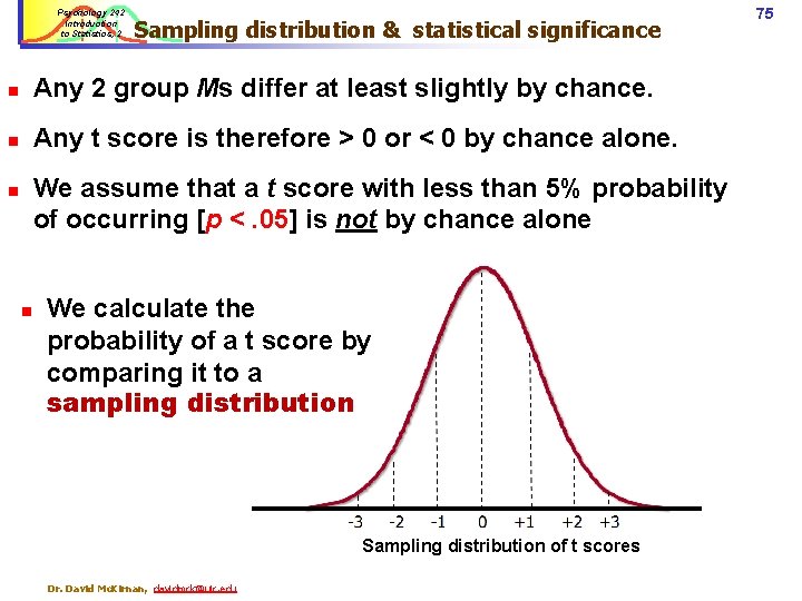
Psychology 242 Introduction to Statistics, 2 Sampling distribution & statistical significance n Any 2 group Ms differ at least slightly by chance. n Any t score is therefore > 0 or < 0 by chance alone. We assume that a t score with less than 5% probability of occurring [p <. 05] is not by chance alone n n We calculate the probability of a t score by comparing it to a sampling distribution Sampling distribution of t scores Dr. David Mc. Kirnan, davidmck@uic. edu 75

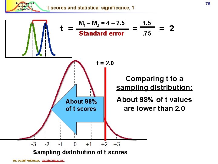
Psychology 242 Introduction to Statistics, 2 76 t scores and statistical significance, 1 t = M 1 – M 2 = 4 – 2. 5 Standard error = 1. 5. 75 = 2 t = 2. 0 Comparing t to a sampling distribution: About 98% of t scores About 98% of t values are lower than 2. 0 Sampling distribution of t scores Dr. David Mc. Kirnan, davidmck@uic. edu

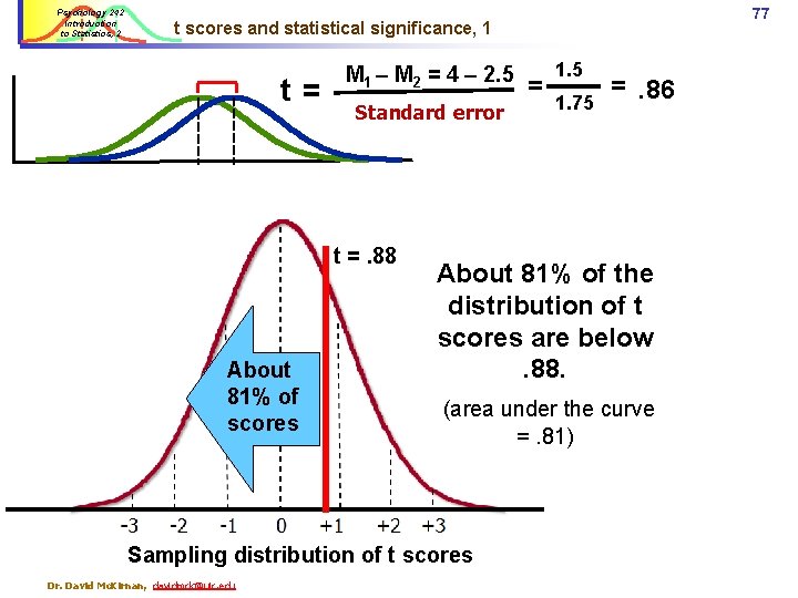
Psychology 242 Introduction to Statistics, 2 77 t scores and statistical significance, 1 t= M 1 – M 2 = 4 – 2. 5 Standard error t =. 88 About 81% of scores 1. 75 =. 86 About 81% of the distribution of t scores are below. 88. (area under the curve =. 81) Sampling distribution of t scores Dr. David Mc. Kirnan, davidmck@uic. edu = 1. 5

Psychology 242 Introduction to Statistics, 2 78 Between v. within group variance: t-test logic The difference between Ms is the same in the two data sets. t =. 86 t = 2. 0 Since the variances differ… ü We get different t values ü We make differ judgments about whether these t scores occurred by chance. Dr. David Mc. Kirnan, davidmck@uic. edu About 98% of t scores; p <. 05 About 81% of scores Sampling distribution of t scores

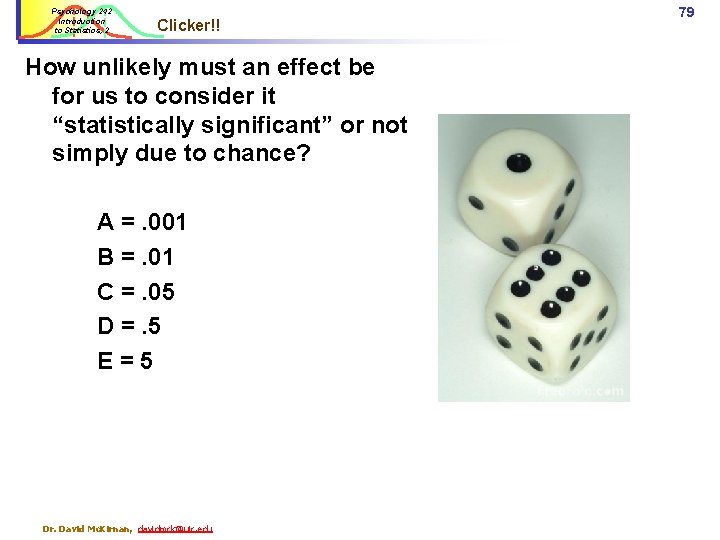
Psychology 242 Introduction to Statistics, 2 Clicker!! How unlikely must an effect be for us to consider it “statistically significant” or not simply due to chance? A =. 001 B =. 01 C =. 05 D =. 5 E=5 Dr. David Mc. Kirnan, davidmck@uic. edu 79

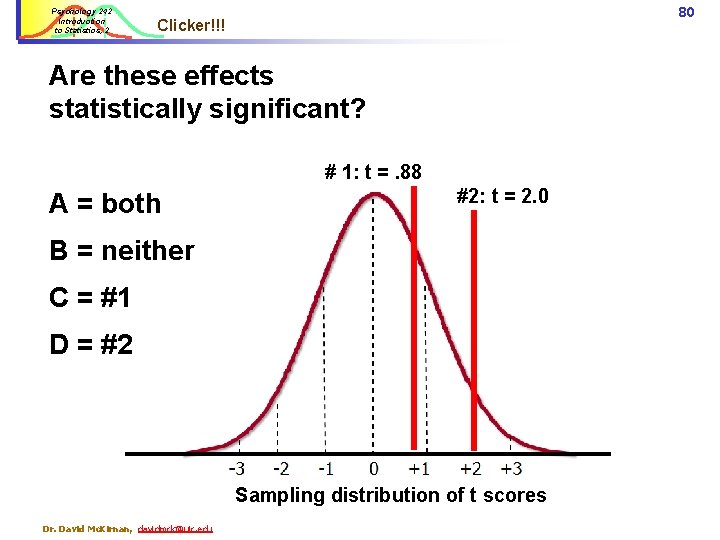
Psychology 242 Introduction to Statistics, 2 80 Clicker!!! Are these effects statistically significant? # 1: t =. 88 A = both #2: t = 2. 0 B = neither C = #1 D = #2 Sampling distribution of t scores Dr. David Mc. Kirnan, davidmck@uic. edu

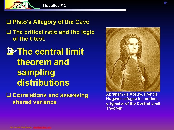
Psychology 242 Introduction to Statistics, 2 81 Statistics # 2 q Plato’s Allegory of the Cave q The critical ratio and the logic of the t-test. The central limit q theorem and sampling distributions q Correlations and assessing shared variance Dr. David Mc. Kirnan, davidmck@uic. edu Abraham de Moivre, French Hugenot refugee in London, originator of the Central Limit Theorem

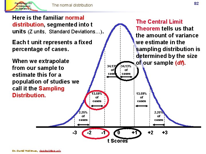
Psychology 242 Introduction to Statistics, 2 82 The normal distribution Here is the familiar normal distribution, segmented into t units (Z units, Standard Deviations…). Each t unit represents a fixed percentage of cases. When we extrapolate from our sample to estimate this for a population of studies we call it the Sampling Distribution. 34. 13% of of cases 13. 59% of cases The Central Limit Theorem tells us that the amount of variance we estimate in the sampling distribution is determined by the size of our sample (df). 13. 59% of cases 2. 25% of cases -3 -2 2. 25% of cases -1 0 t Scores Dr. David Mc. Kirnan, davidmck@uic. edu +1 +2 +3

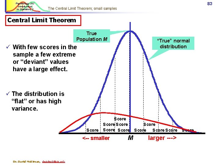
Psychology 242 Introduction to Statistics, 2 83 The Central Limit Theorem; small samples Central Limit Theorem True Population M “True” normal distribution ü With few scores in the sample a few extreme or “deviant” values have a large effect. ü The distribution is “flat” or has high variance. Score Score <-- smaller Dr. David Mc. Kirnan, davidmck@uic. edu M Score larger ---> Score

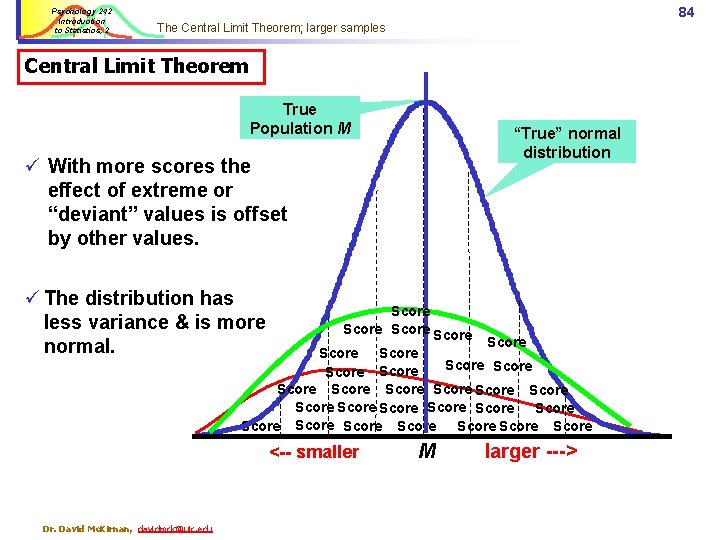
Psychology 242 Introduction to Statistics, 2 84 The Central Limit Theorem; larger samples Central Limit Theorem True Population M “True” normal distribution ü With more scores the effect of extreme or “deviant” values is offset by other values. ü The distribution has less variance & is more normal. Score Score Score Score Score Score Score Score <-- smaller Dr. David Mc. Kirnan, davidmck@uic. edu M larger --->

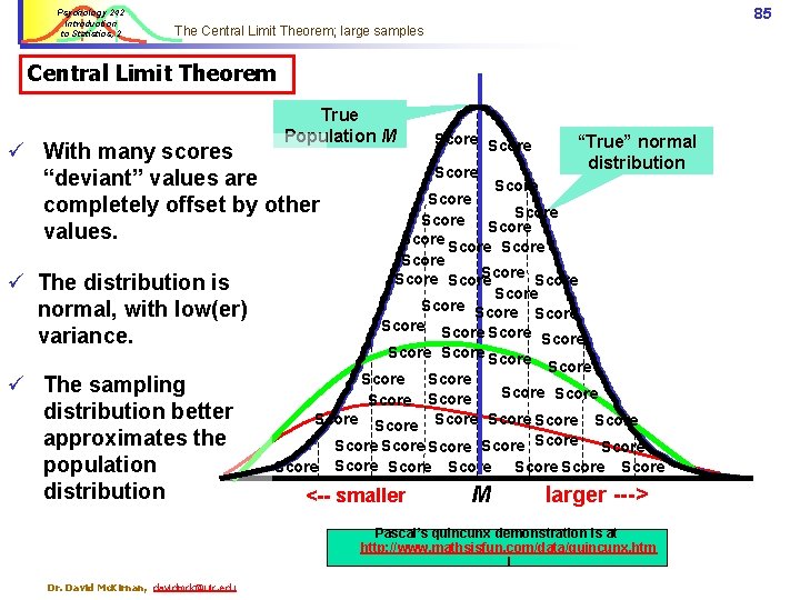
Psychology 242 Introduction to Statistics, 2 85 The Central Limit Theorem; large samples Central Limit Theorem True Population M ü With many scores “deviant” values are completely offset by other values. ü The distribution is normal, with low(er) variance. ü The sampling distribution better approximates the population distribution Score “True” normal distribution Score Score Score Score Score Score Score Score Score Score Score Score <-- smaller Score M Score larger ---> Pascal’s quincunx demonstration is at http: //www. mathsisfun. com/data/quincunx. htm l Dr. David Mc. Kirnan, davidmck@uic. edu

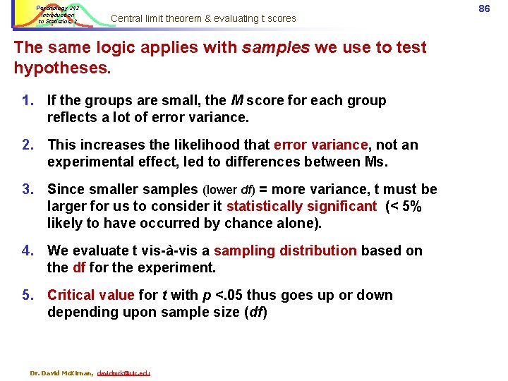
Psychology 242 Introduction to Statistics, 2 Central limit theorem & evaluating t scores The same logic applies with samples we use to test hypotheses. 1. If the groups are small, the M score for each group reflects a lot of error variance. 2. This increases the likelihood that error variance, not an experimental effect, led to differences between Ms. 3. Since smaller samples (lower df) = more variance, t must be larger for us to consider it statistically significant (< 5% likely to have occurred by chance alone). 4. We evaluate t vis-à-vis a sampling distribution based on the df for the experiment. 5. Critical value for t with p <. 05 thus goes up or down depending upon sample size (df) Dr. David Mc. Kirnan, davidmck@uic. edu 86

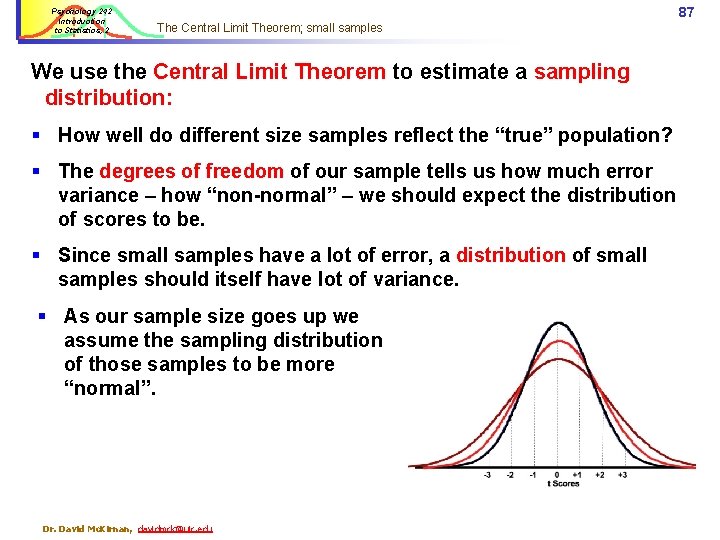
Psychology 242 Introduction to Statistics, 2 87 The Central Limit Theorem; small samples We use the Central Limit Theorem to estimate a sampling distribution: § How well do different size samples reflect the “true” population? § The degrees of freedom of our sample tells us how much error variance – how “non-normal” – we should expect the distribution of scores to be. § Since small samples have a lot of error, a distribution of small samples should itself have lot of variance. § As our sample size goes up we assume the sampling distribution of those samples to be more “normal”. Dr. David Mc. Kirnan, davidmck@uic. edu

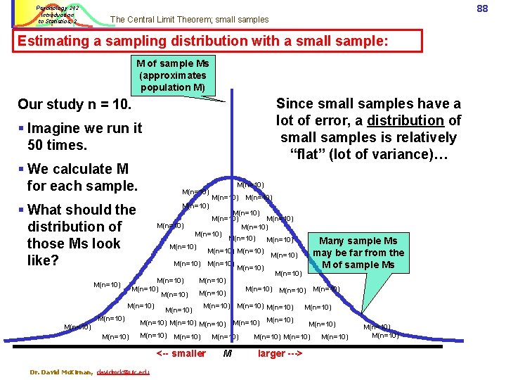
Psychology 242 Introduction to Statistics, 2 88 The Central Limit Theorem; small samples Estimating a sampling distribution with a small sample: M of sample Ms (approximates population M) Since small samples have a lot of error, a distribution of small samples is relatively “flat” (lot of variance)… Our study n = 10. § Imagine we run it 50 times. § We calculate M for each sample. M(n=10) § What should the distribution of those Ms look like? M(n=10) M(n=10) M(n=10) Many sample Ms M(n=10) may be far from the M(n=10) M of sample Ms M(n=10) M(n=10) M(n=10) M(n=10) M(n=10) M(n=10) M(n=10) <-- smaller Dr. David Mc. Kirnan, davidmck@uic. edu M(n=10) M(n=10) larger ---> M(n=10)

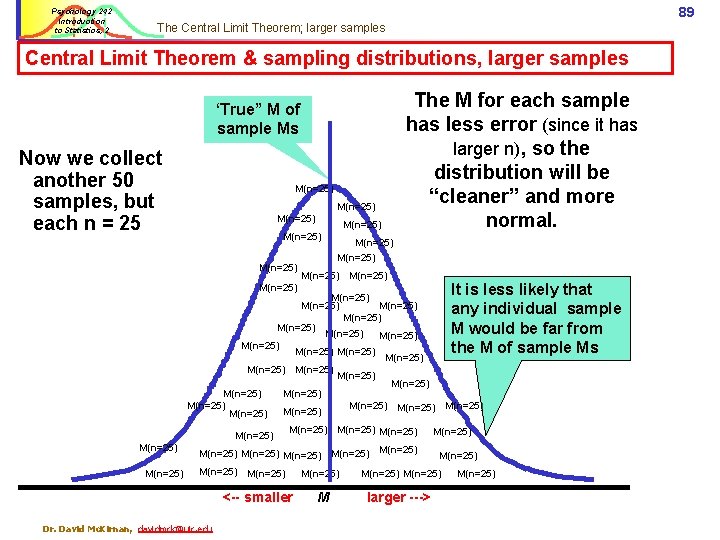
Psychology 242 Introduction to Statistics, 2 89 The Central Limit Theorem; larger samples Central Limit Theorem & sampling distributions, larger samples ‘True” M of sample Ms Now we collect another 50 samples, but each n = 25 M(n=25) M(n=25) The M for each sample has less error (since it has larger n), so the distribution will be “cleaner” and more normal. M(n=25) It is less likely that any individual sample M would be far from the M of sample Ms M(n=25) M(n=25) M(n=25) M(n=25) M(n=25) M(n=25) M(n=25) M(n=25) M(n=25) M(n=25) <-- smaller Dr. David Mc. Kirnan, davidmck@uic. edu M(n=25) M(n=25) larger ---> M(n=25)

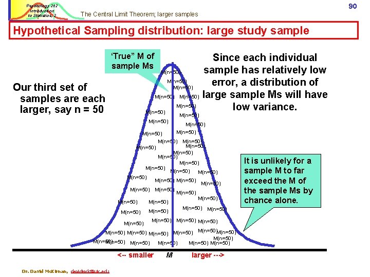
Psychology 242 Introduction to Statistics, 2 90 The Central Limit Theorem; larger samples Hypothetical Sampling distribution: large study sample ‘True” M of sample Ms M(n=50) Our third set of samples are each larger, say n = 50 M(n=50) Since each individual sample has relatively low error, a distribution of large sample Ms will have low variance. M(n=50) M(n=50) M(n=50) M(n=50) M(n=50) M(n=50) M(n=50) M(n=50) M(n=50) M(n=50)M(n=50) M(n=50) <-- smaller Dr. David Mc. Kirnan, davidmck@uic. edu M larger ---> It is unlikely for a sample M to far exceed the M of the sample Ms by chance alone.

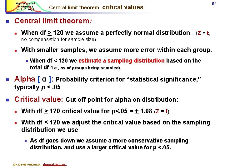
Psychology 242 Introduction to Statistics, 2 n Central limit theorem: critical 91 values Central limit theorem: n When df > 120 we assume a perfectly normal distribution. (Z = t; no compensation for sample size) n With smaller samples, we assume more error within each group. n n When df < 120 we estimate a sampling distribution based on the total df (i. e. , ns of groups being sampled). Alpha [ α ]: Probability criterion for “statistical significance, ” typically p <. 05 n Critical value: Cut off point for alpha on distribution: n n With df > 120 critical value for p<. 05 = + 1. 98 (Z = t) With df < 120 we adjust the critical value based on the sampling distribution we use n As df goes down we assume a more conservative sampling distribution, and use a larger critical value for p <. 05. Dr. David Mc. Kirnan, davidmck@uic. edu

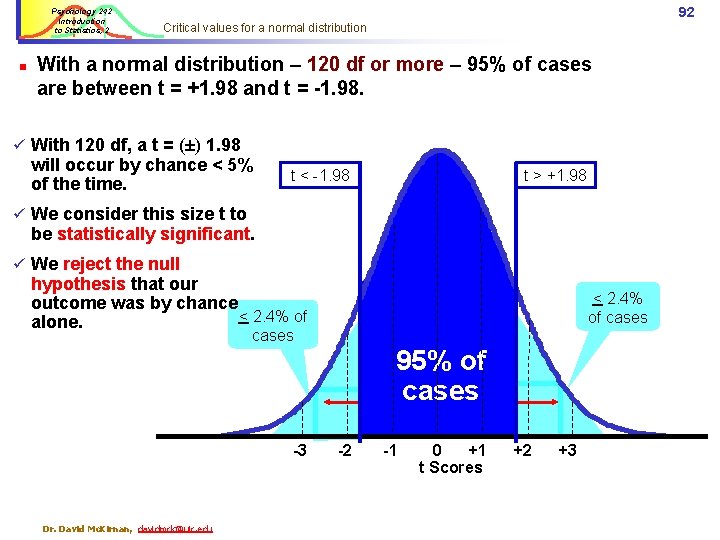
Psychology 242 Introduction to Statistics, 2 n 92 Critical values for a normal distribution With a normal distribution – 120 df or more – 95% of cases are between t = +1. 98 and t = -1. 98. ü With 120 df, a t = (±) 1. 98 will occur by chance < 5% of the time. t < -1. 98 t > +1. 98 ü We consider this size t to be statistically significant. ü We reject the null hypothesis that our outcome was by chance < 2. 4% of alone. < 2. 4% of cases 95% of cases -3 Dr. David Mc. Kirnan, davidmck@uic. edu -2 -1 0 +1 t Scores +2 +3

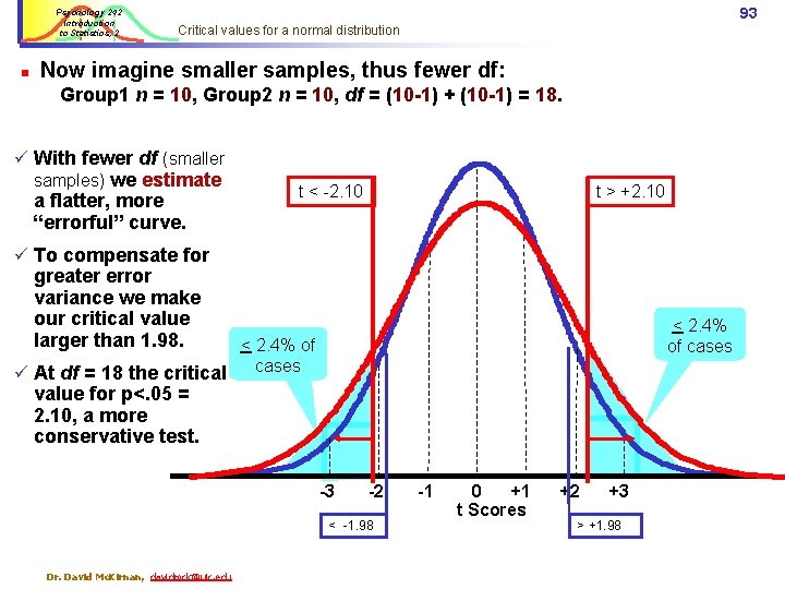
Psychology 242 Introduction to Statistics, 2 n 93 Critical values for a normal distribution Now imagine smaller samples, thus fewer df: Group 1 n = 10, Group 2 n = 10, df = (10 -1) + (10 -1) = 18. ü With fewer df (smaller samples) we estimate a flatter, more “errorful” curve. t < -2. 10 t > +2. 10 ü To compensate for greater error variance we make our critical value larger than 1. 98. < 2. 4% of cases ü At df = 18 the critical value for p<. 05 = 2. 10, a more conservative test. -3 -2 < -1. 98 Dr. David Mc. Kirnan, davidmck@uic. edu -1 0 +1 t Scores +2 +3 > +1. 98

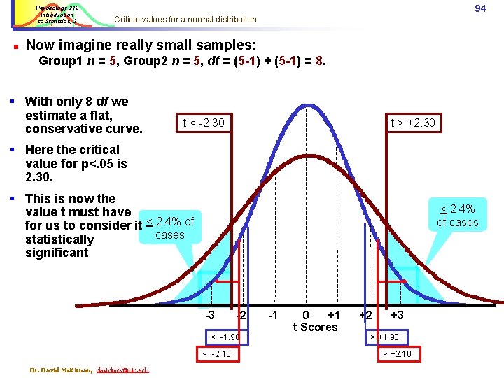
Psychology 242 Introduction to Statistics, 2 n 94 Critical values for a normal distribution Now imagine really small samples: Group 1 n = 5, Group 2 n = 5, df = (5 -1) + (5 -1) = 8. § With only 8 df we estimate a flat, conservative curve. t < -2. 30 t > +2. 30 § Here the critical value for p<. 05 is 2. 30. § This is now the value t must have for us to consider it < 2. 4% of cases statistically significant < 2. 4% of cases -3 -2 < -1. 98 < -2. 10 Dr. David Mc. Kirnan, davidmck@uic. edu -1 0 +1 t Scores +2 +3 > +1. 98 > +2. 10

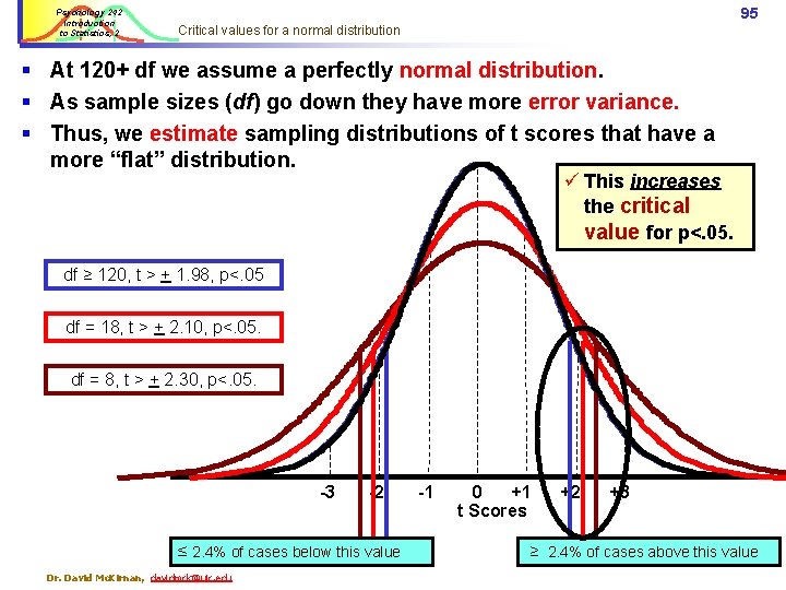
Psychology 242 Introduction to Statistics, 2 95 Critical values for a normal distribution § At 120+ df we assume a perfectly normal distribution. § As sample sizes (df) go down they have more error variance. § Thus, we estimate sampling distributions of t scores that have a more “flat” distribution. ü This increases the critical value for p<. 05. df ≥ 120, t > + 1. 98, p<. 05 df = 18, t > + 2. 10, p<. 05. df = 8, t > + 2. 30, p<. 05. -3 -2 ≤ 2. 4% of cases below this value Dr. David Mc. Kirnan, davidmck@uic. edu -1 0 +1 t Scores +2 +3 ≥ 2. 4% of cases above this value

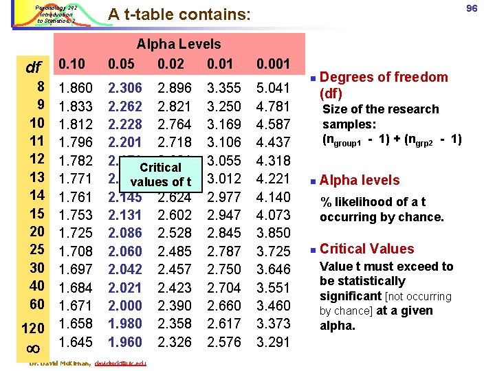
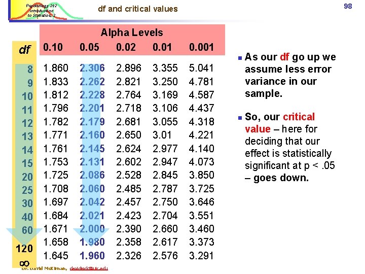
Psychology 242 Introduction to Statistics, 2 df 0. 10 8 9 10 11 12 13 14 15 20 25 30 40 60 1. 833 1. 812 1. 796 1. 782 1. 771 1. 761 1. 753 1. 725 1. 708 1. 697 1. 684 1. 671 1. 658 1. 645 120 96 A t-table contains: Alpha Levels 0. 05 0. 02 0. 01 2. 306 2. 896 2. 262 2. 821 2. 228 2. 764 2. 201 2. 718 2. 179 Critical 2. 681 2. 160 2. 650 values of t 2. 145 2. 624 2. 131 2. 602 2. 086 2. 528 2. 060 2. 485 2. 042 2. 457 2. 021 2. 423 2. 000 2. 390 1. 980 2. 358 1. 960 2. 326 Dr. David Mc. Kirnan, davidmck@uic. edu 3. 355 3. 250 3. 169 3. 106 3. 055 3. 012 2. 977 2. 947 2. 845 2. 787 2. 750 2. 704 2. 660 2. 617 2. 576 0. 001 5. 041 4. 781 4. 587 4. 437 4. 318 4. 221 4. 140 4. 073 3. 850 3. 725 3. 646 3. 551 3. 460 3. 373 3. 291 n Degrees of freedom (df) Size of the research samples: (ngroup 1 - 1) + (ngrp 2 - 1) n Alpha levels % likelihood of a t occurring by chance. n Critical Values Value t must exceed to be statistically significant [not occurring by chance] at a given alpha.

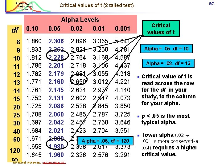
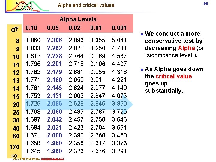
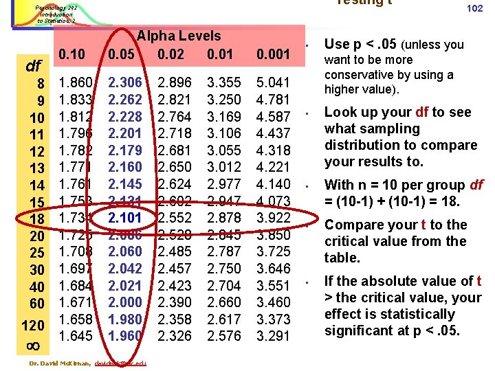
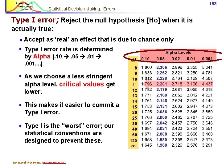
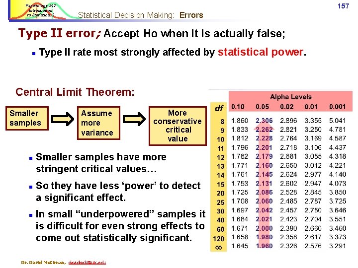
Psychology 242 Introduction to Statistics, 2 df 0. 10 Alpha Levels 0. 05 0. 02 0. 01 8 9 10 11 12 13 14 15 20 25 30 40 60 1. 833 1. 812 1. 796 1. 782 1. 771 1. 761 1. 753 1. 725 1. 708 1. 697 1. 684 1. 671 1. 658 1. 645 2. 306 2. 262 2. 228 2. 201 2. 179 2. 160 2. 145 2. 131 2. 086 2. 060 2. 042 2. 021 2. 000 1. 980 1. 960 120 97 Critical values of t (2 tailed test) Dr. David Mc. Kirnan, davidmck@uic. edu Critical values of t 0. 001 2. 896 3. 355 5. 041 2. 821 3. 250 4. 781 2. 764 3. 169 4. 587 2. 718 3. 106 4. 437 2. 681 3. 055 4. 318 2. 650 3. 012 4. 221 2. 624 2. 977 4. 140 2. 602 2. 947 4. 073 2. 528 2. 845 3. 850 2. 485 2. 787 3. 725 2. 457 2. 750 3. 646 2. 423 2. 704 3. 551 2. 390 2. 660 Alpha =. 05, df 3. 460 = 120 2. 358 2. 617 3. 373 2. 326 2. 576 3. 291 Alpha =. 05, df = 10 Alpha =. 02, df = 13 n n n Critical value of t is read across the row for the df in your study, to the column for your alpha. p <. 05 is the most typical alpha. lower alpha (. 02 . 001, a more conservative test) requires a higher critical value.

Psychology 242 Introduction to Statistics, 2 df 0. 10 8 9 10 11 12 13 14 15 20 25 30 40 60 1. 833 1. 812 1. 796 1. 782 1. 771 1. 761 1. 753 1. 725 1. 708 1. 697 1. 684 1. 671 1. 658 1. 645 120 98 df and critical values Alpha Levels 0. 05 0. 02 0. 01 0. 001 n 2. 306 2. 262 2. 228 2. 201 2. 179 2. 160 2. 145 2. 131 2. 086 2. 060 2. 042 2. 021 2. 000 1. 980 1. 960 Dr. David Mc. Kirnan, davidmck@uic. edu 2. 896 2. 821 2. 764 2. 718 2. 681 2. 650 2. 624 2. 602 2. 528 2. 485 2. 457 2. 423 2. 390 2. 358 2. 326 3. 355 3. 250 3. 169 3. 106 3. 055 3. 01 2. 977 2. 947 2. 845 2. 787 2. 750 2. 704 2. 660 2. 617 2. 576 5. 041 4. 781 4. 587 4. 437 4. 318 4. 221 4. 140 4. 073 3. 850 3. 725 3. 646 3. 551 3. 460 3. 373 3. 291 n As our df go up we assume less error variance in our sample. So, our critical value – here for deciding that our effect is statistically significant at p <. 05 – goes down.

Psychology 242 Introduction to Statistics, 2 df 0. 10 8 9 10 11 12 13 14 15 20 25 30 40 60 1. 833 1. 812 1. 796 1. 782 1. 771 1. 761 1. 753 1. 725 1. 708 1. 697 1. 684 1. 671 1. 658 1. 645 120 99 Alpha and critical values Alpha Levels 0. 05 0. 02 0. 01 0. 001 n 2. 306 2. 262 2. 228 2. 201 2. 179 2. 160 2. 145 2. 131 2. 086 2. 060 2. 042 2. 021 2. 000 1. 980 1. 960 Dr. David Mc. Kirnan, davidmck@uic. edu 2. 896 2. 821 2. 764 2. 718 2. 681 2. 650 2. 624 2. 602 2. 528 2. 485 2. 457 2. 423 2. 390 2. 358 2. 326 3. 355 3. 250 3. 169 3. 106 3. 055 3. 01 2. 977 2. 947 2. 845 2. 787 2. 750 2. 704 2. 660 2. 617 2. 576 5. 041 4. 781 4. 587 4. 437 4. 318 4. 221 4. 140 4. 073 3. 850 3. 725 3. 646 3. 551 3. 460 3. 373 3. 291 n We conduct a more conservative test by decreasing Alpha (or “significance level”). As Alpha goes down the critical value goes up substantially.

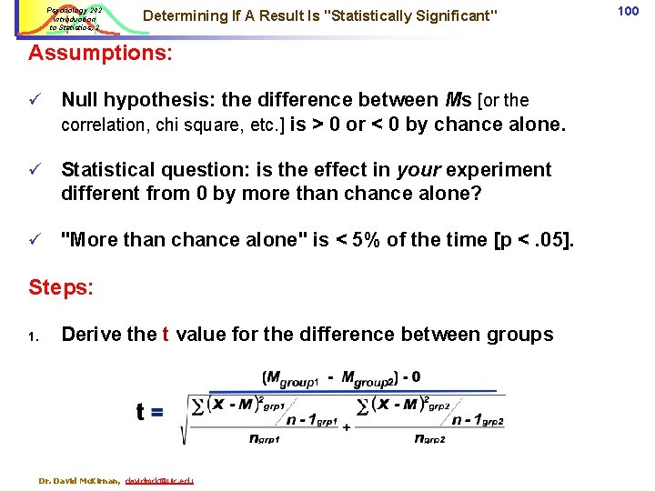
Psychology 242 Introduction to Statistics, 2 Determining If A Result Is "Statistically Significant" Assumptions: ü Null hypothesis: the difference between Ms [or the correlation, chi square, etc. ] is > 0 or < 0 by chance alone. ü Statistical question: is the effect in your experiment different from 0 by more than chance alone? ü "More than chance alone" is < 5% of the time [p <. 05]. Steps: 1. Derive the t value for the difference between groups Dr. David Mc. Kirnan, davidmck@uic. edu 100

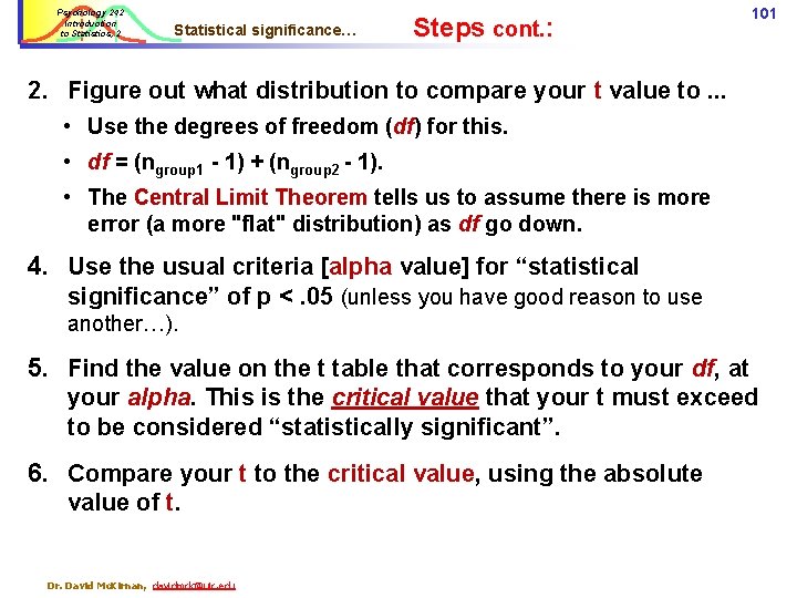
Psychology 242 Introduction to Statistics, 2 Statistical significance… Steps cont. : 101 2. Figure out what distribution to compare your t value to. . . • Use the degrees of freedom (df) for this. • df = (ngroup 1 - 1) + (ngroup 2 - 1). • The Central Limit Theorem tells us to assume there is more error (a more "flat" distribution) as df go down. 4. Use the usual criteria [alpha value] for “statistical significance” of p <. 05 (unless you have good reason to use another…). 5. Find the value on the t table that corresponds to your df, at your alpha. This is the critical value that your t must exceed to be considered “statistically significant”. 6. Compare your t to the critical value, using the absolute value of t. Dr. David Mc. Kirnan, davidmck@uic. edu

Testing t Psychology 242 Introduction to Statistics, 2 df 8 9 10 11 12 13 14 15 18 20 25 30 40 60 120 0. 10 Alpha Levels 0. 05 0. 02 0. 01 0. 001 1. 860 1. 833 1. 812 1. 796 1. 782 1. 771 1. 761 1. 753 1. 734 1. 725 1. 708 1. 697 1. 684 1. 671 1. 658 1. 645 2. 306 2. 262 2. 228 2. 201 2. 179 2. 160 2. 145 2. 131 2. 101 2. 086 2. 060 2. 042 2. 021 2. 000 1. 980 1. 960 5. 041 4. 781 4. 587 4. 437 4. 318 4. 221 4. 140 4. 073 3. 922 3. 850 3. 725 3. 646 3. 551 3. 460 3. 373 3. 291 Dr. David Mc. Kirnan, davidmck@uic. edu 2. 896 2. 821 2. 764 2. 718 2. 681 2. 650 2. 624 2. 602 2. 552 2. 528 2. 485 2. 457 2. 423 2. 390 2. 358 2. 326 3. 355 3. 250 3. 169 3. 106 3. 055 3. 012 2. 977 2. 947 2. 878 2. 845 2. 787 2. 750 2. 704 2. 660 2. 617 2. 576 • 102 Use p <. 05 (unless you want to be more conservative by using a higher value). • • Look up your df to see what sampling distribution to compare your results to. With n = 10 per group df = (10 -1) + (10 -1) = 18. Compare your t to the critical value from the table. If the absolute value of t > the critical value, your effect is statistically significant at p <. 05.

Psychology 242 Introduction to Statistics, 2 Statistics # 2 q Plato’s Allegory of the Cave q The critical ratio and the logic of the t-test. q The central limit theorem and sampling distributions Correlations and q assessing shared variance Dr. David Mc. Kirnan, davidmck@uic. edu 103

Psychology 242 Introduction to Statistics, 2 Testing a hypothesis: t-test versus correlation How much do you love statistics? A = Completely B = A lot C = Pretty much D = Just a little E = Not at all Dr. David Mc. Kirnan, davidmck@uic. edu 104

Psychology 242 Introduction to Statistics, 2 105 t-test versus correlation How are you doing in statistics? A = Terrific B = Good C = OK D = Getting by E = Not so good Dr. David Mc. Kirnan, davidmck@uic. edu

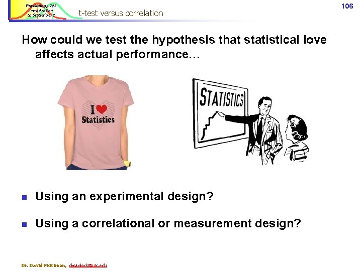
Psychology 242 Introduction to Statistics, 2 t-test versus correlation How could we test the hypothesis that statistical love affects actual performance… n Using an experimental design? n Using a correlational or measurement design? Dr. David Mc. Kirnan, davidmck@uic. edu 106

Psychology 242 Introduction to Statistics, 2 n t-tests: n n Used for experiments Manipulate the independent variable n n Exciting versus “placebo” material. Measure differences in the Dependent Variable. n n Testing a hypothesis: t-test versus correlation Psychology 242 grade. Correlations: n Used for measurement studies n Measure the Predictor variable n n How much do people love statistics Measure the Outcome variable n Psychology 242 grade. Dr. David Mc. Kirnan, davidmck@uic. edu 107

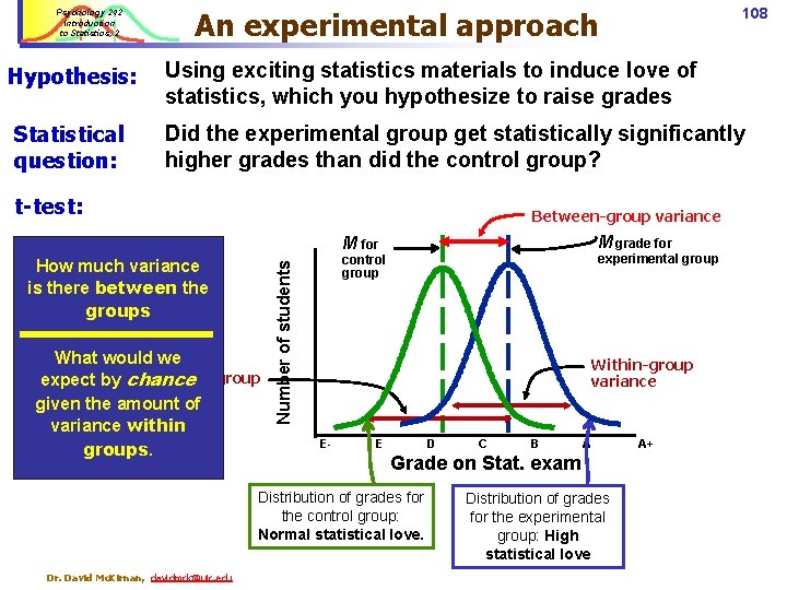
Psychology 242 Introduction to Statistics, 2 108 An experimental approach Hypothesis: Using exciting statistics materials to induce love of statistics, which you hypothesize to raise grades Statistical question: Did the experimental group get statistically significantly higher grades than did the control group? t-test: Between-group variance M grade for M for What would we Within-group expect by chance variance given the amount of variance within groups. experimental group control group Number of students How much variance is there between the groups Within-group variance E- E D B A Grade on Stat. exam Distribution of grades for the control group: Normal statistical love. Dr. David Mc. Kirnan, davidmck@uic. edu C Distribution of grades for the experimental group: High statistical love A+

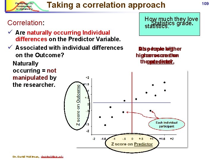
Psychology 242 Introduction to Statistics, 2 Taking a correlation approach Correlation: ü Are naturally occurring Individual differences on the Predictor Variable. ü Associated with individual differences on the Outcome? Naturally occurring = not manipulated by the researcher. Dr. David Mc. Kirnan, davidmck@uic. edu How much they love Statistics grade. statistics. Also Do people have higher with higher scores on theoutcome? predictor, 109

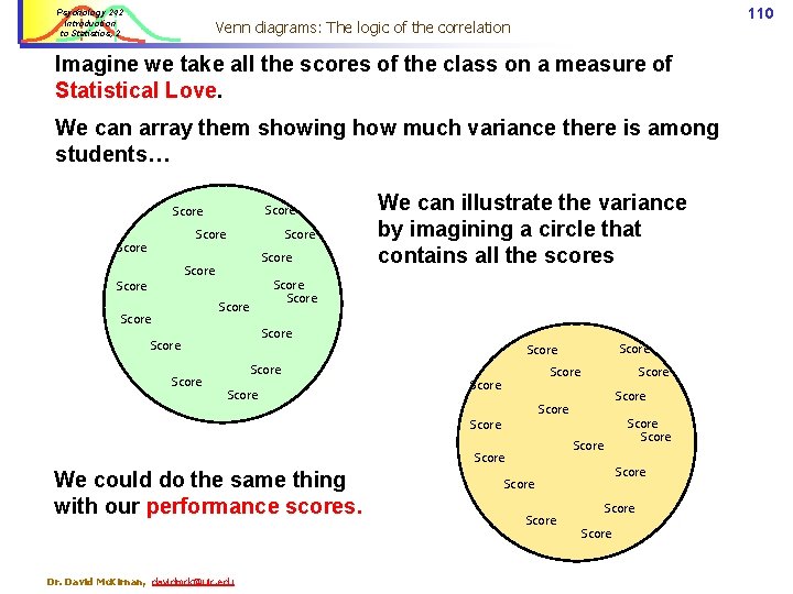
Psychology 242 Introduction to Statistics, 2 110 Venn diagrams: The logic of the correlation Imagine we take all the scores of the class on a measure of Statistical Love. We can array them showing how much variance there is among students… Score Score Score Score We can illustrate the variance by imagining a circle that contains all the scores Score Score Score Dr. David Mc. Kirnan, davidmck@uic. edu Score We could do the same thing with our performance scores. Score Score

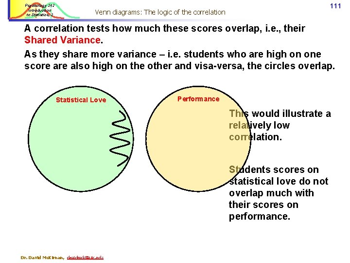
Psychology 242 Introduction to Statistics, 2 111 Venn diagrams: The logic of the correlation A correlation tests how much these scores overlap, i. e. , their Shared Variance. As they share more variance – i. e. students who are high on one score also high on the other and visa-versa, the circles overlap. Statistical Love Performance This would illustrate a relatively low correlation. Students scores on statistical love do not overlap much with their scores on performance. Dr. David Mc. Kirnan, davidmck@uic. edu

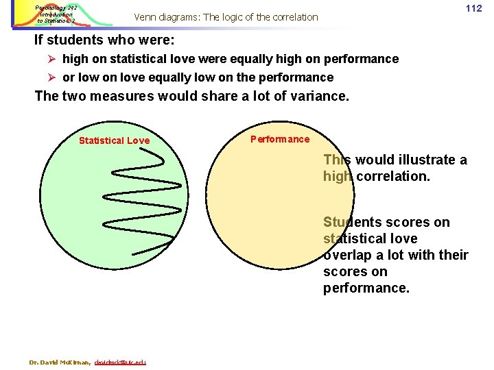
Psychology 242 Introduction to Statistics, 2 112 Venn diagrams: The logic of the correlation If students who were: Ø high on statistical love were equally high on performance Ø or low on love equally low on the performance The two measures would share a lot of variance. Statistical Love Performance This would illustrate a high correlation. Students scores on statistical love overlap a lot with their scores on performance. Dr. David Mc. Kirnan, davidmck@uic. edu

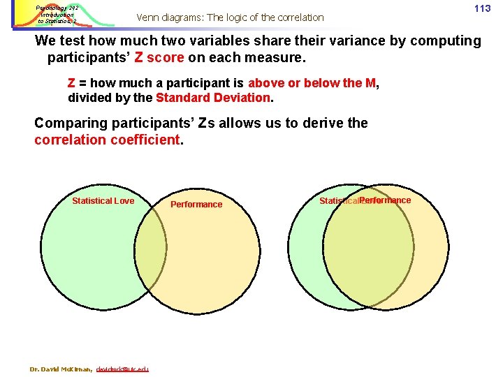
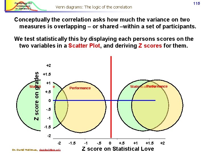
Psychology 242 Introduction to Statistics, 2 Venn diagrams: The logic of the correlation 113 We test how much two variables share their variance by computing participants’ Z score on each measure. Z = how much a participant is above or below the M, divided by the Standard Deviation. Comparing participants’ Zs allows us to derive the correlation coefficient. Statistical Love Dr. David Mc. Kirnan, davidmck@uic. edu Performance Statistical Performance Love

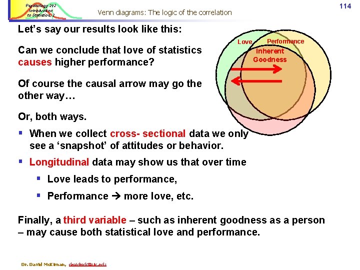
Psychology 242 Introduction to Statistics, 2 114 Venn diagrams: The logic of the correlation Let’s say our results look like this: Can we conclude that love of statistics causes higher performance? Love Performance Inherent Goodness Of course the causal arrow may go the other way… Or, both ways. § When we collect cross- sectional data we only see a ‘snapshot’ of attitudes or behavior. § Longitudinal data may show us that over time § Love leads to performance, § Performance more love, etc. Finally, a third variable – such as inherent goodness as a person – may cause both statistical love and performance. Dr. David Mc. Kirnan, davidmck@uic. edu

Psychology 242 Introduction to Statistics, 2 115 Venn diagrams: The logic of the correlation Conceptually the correlation asks how much the variance on two measures is overlapping – or shared –within a set of participants. We test statistically this by displaying each persons scores on the two variables in a Scatter Plot, and deriving Z scores for them. Z score on grades +2 +1. 5 +1 Statistical Love Statistical Performance Love Performance +. 5 0 -. 5 -1 -1. 5 -2 -2 Dr. David Mc. Kirnan, davidmck@uic. edu -1. 5 -1 -. 5 0 +. 5 +1 +1. 5 Z score on Statistical Love +2

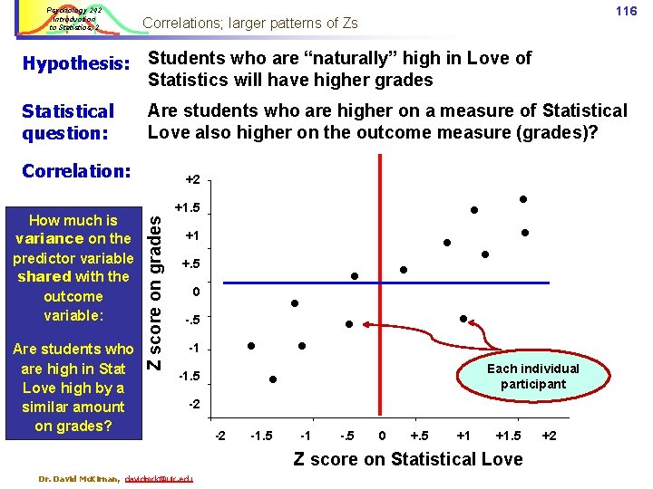
Psychology 242 Introduction to Statistics, 2 116 Correlations; larger patterns of Zs Hypothesis: Students who are “naturally” high in Love of Statistics will have higher grades Statistical question: Are students who are higher on a measure of Statistical Love also higher on the outcome measure (grades)? Correlation: Are students who are high in Stat Love high by a similar amount on grades? +1. 5 Z score on grades How much is variance on the predictor variable shared with the outcome variable: +2 +1 +. 5 0 -. 5 -1 Each individual participant -1. 5 -2 -2 -1. 5 -1 -. 5 0 +. 5 +1 +1. 5 Z score on Statistical Love Dr. David Mc. Kirnan, davidmck@uic. edu +2

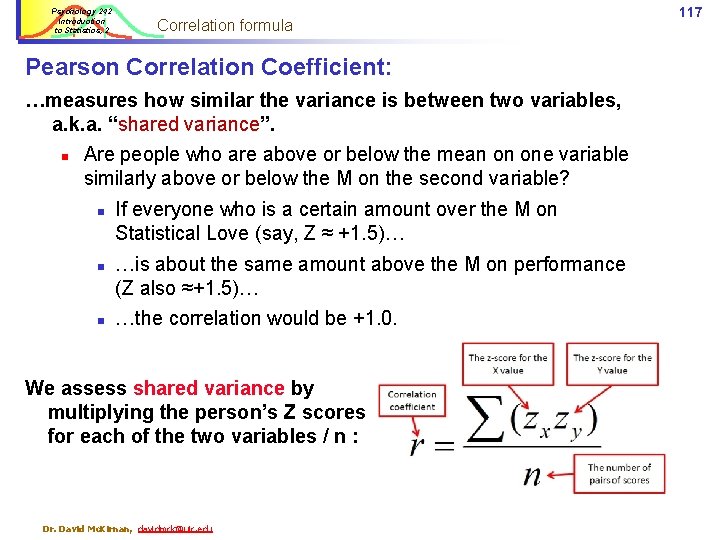
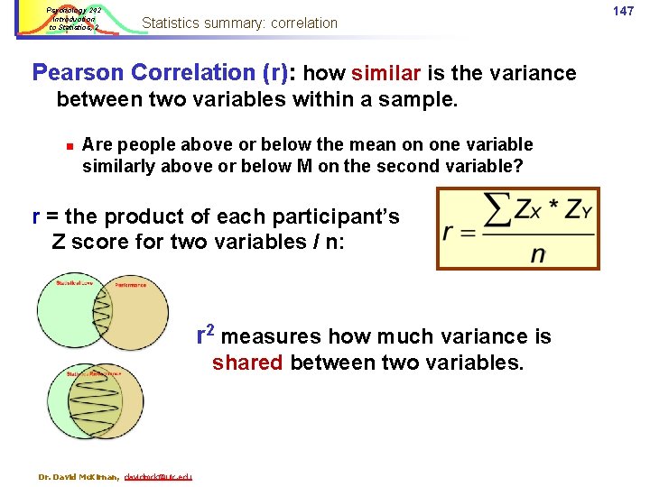
Psychology 242 Introduction to Statistics, 2 Correlation formula Pearson Correlation Coefficient: …measures how similar the variance is between two variables, a. k. a. “shared variance”. n Are people who are above or below the mean on one variable similarly above or below the M on the second variable? n n n If everyone who is a certain amount over the M on Statistical Love (say, Z ≈ +1. 5)… …is about the same amount above the M on performance (Z also ≈+1. 5)… …the correlation would be +1. 0. We assess shared variance by multiplying the person’s Z scores for each of the two variables / n : Dr. David Mc. Kirnan, davidmck@uic. edu 117

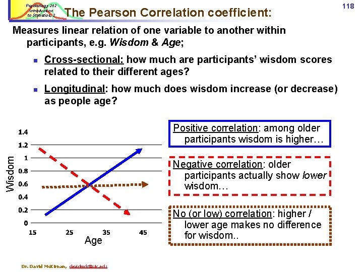
Psychology 242 Introduction to Statistics, 2 The Pearson Correlation coefficient: Measures linear relation of one variable to another within participants, e. g. Wisdom & Age; n n Cross-sectional: how much are participants’ wisdom scores related to their different ages? Longitudinal: how much does wisdom increase (or decrease) as people age? Wisdom Positive correlation: among older participants wisdom is higher… Negative correlation: older participants actually show lower wisdom… Age Dr. David Mc. Kirnan, davidmck@uic. edu No (or low) correlation: higher / lower age makes no difference for wisdom. . 118

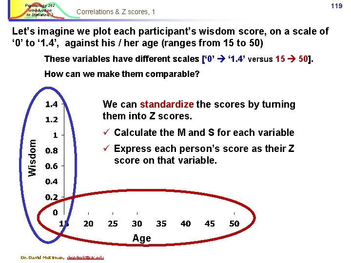
Psychology 242 Introduction to Statistics, 2 Correlations & Z scores, 1 Let’s imagine we plot each participant’s wisdom score, on a scale of ‘ 0’ to ‘ 1. 4’, against his / her age (ranges from 15 to 50) These variables have different scales [‘ 0’ ‘ 1. 4’ versus 15 50]. How can we make them comparable? We can standardize the scores by turning them into Z scores. Wisdom ü Calculate the M and S for each variable ü Express each person’s score as their Z score on that variable. Age Dr. David Mc. Kirnan, davidmck@uic. edu 119

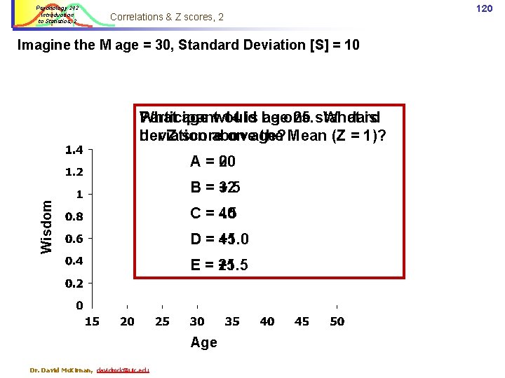
Psychology 242 Introduction to Statistics, 2 Correlations & Z scores, 2 Imagine the M age = 30, Standard Deviation [S] = 10 Participant What age would 14 is be ageone 25. standard What is deviation her Z score above on age? the Mean (Z = 1)? A=0 20 Wisdom B = +. 5 32 C = -. 5 40 D = +1. 0 45 E = +1. 5 25 Age Dr. David Mc. Kirnan, davidmck@uic. edu 120

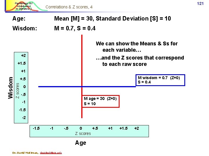
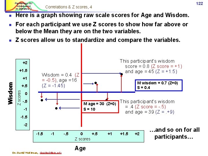
Psychology 242 Introduction to Statistics, 2 121 Correlations & Z scores, 4 Age: Mean [M] = 30, Standard Deviation [S] = 10 Wisdom: M = 0. 7, S = 0. 4 We can show the Means & Ss for each variable… +2 …and the Z scores that correspond to each raw score +1. 5 M wisdom = 0. 7 (Z=0) S = 0. 4 +. 5 Z scores Wisdom +1 0 -. 5 M age = 30 (Z=0) S = 10 -1 -1. 5 -2 -1. 5 -1 -. 5 0 +. 5 Z scores Age Dr. David Mc. Kirnan, davidmck@uic. edu +1 +1. 5 +2

Psychology 242 Introduction to Statistics, 2 122 Correlations & Z scores, 4 Here is a graph showing raw scale scores for Age and Wisdom. n For each participant we use Z scores to show far above or below the Mean they are on the two variables. n Z scores allow us to standardize and compare the variables. n This participant’s wisdom score = 0. 8 (Z score = +1) and age = 45 (Z = +1. 5) +2 +1. 5 +. 5 Z scores Wisdom +1 0 -. 5 Wisdom = 0. 4 (Z = -0. 5), age =16 (Z = -1. 45) M wisdom = 0. 7 (Z=0) S = 0. 4 M age = 30 (Z=0) S = 10 -1 This participant’s wisdom =. 4 (Z score = -. 5) and age = 39 (Z =. +9) -1. 5 -2 -1. 5 -1 Dr. David Mc. Kirnan, davidmck@uic. edu -. 5 0 +. 5 Z scores Age +1 +1. 5 +2 …and so on for all participants…

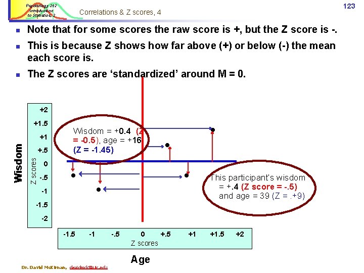
Psychology 242 Introduction to Statistics, 2 123 Correlations & Z scores, 4 Note that for some scores the raw score is +, but the Z score is -. n This is because Z shows how far above (+) or below (-) the mean each score is. n The Z scores are ‘standardized’ around M = 0. n +2 +1. 5 +. 5 Z scores Wisdom +1 0 -. 5 Wisdom = +0. 4 (Z = -0. 5), age = +16 (Z = -1. 45) -1 This participant’s wisdom = +. 4 (Z score = -. 5) and age = 39 (Z =. +9) -1. 5 -2 -1. 5 -1 Dr. David Mc. Kirnan, davidmck@uic. edu -. 5 0 +. 5 Z scores Age +1 +1. 5 +2

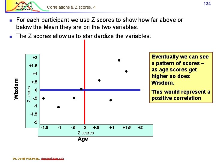
Psychology 242 Introduction to Statistics, 2 The Z scores allow us to standardize the variables. +2 +1 +. 5 0 -. 5 Eventually we can see a pattern of scores – as age scores get higher so does Wisdom. +1. 5 Z scores n For each participant we use Z scores to show far above or below the Mean they are on the two variables. Wisdom n 124 Correlations & Z scores, 4 -1 -1. 5 This would represent a positive correlation -2 -1. 5 -1 -. 5 0 +. 5 Z scores Age Dr. David Mc. Kirnan, davidmck@uic. edu +1 +1. 5 +2

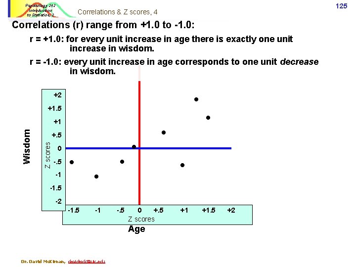
Psychology 242 Introduction to Statistics, 2 125 Correlations & Z scores, 4 Correlations (r) range from +1. 0 to -1. 0: r = +1. 0: for every unit increase in age there is exactly one unit increase in wisdom. r = -1. 0: every unit increase in age corresponds to one unit decrease in wisdom. +2 +1. 5 +. 5 Z scores Wisdom +1 0 -. 5 -1 -1. 5 -2 -1. 5 -1 -. 5 0 +. 5 Z scores Age Dr. David Mc. Kirnan, davidmck@uic. edu +1 +1. 5 +2

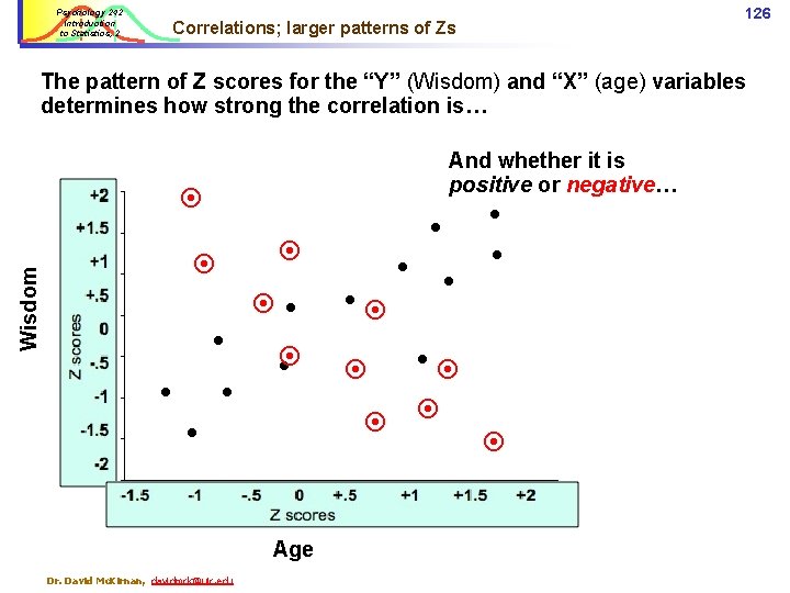
Psychology 242 Introduction to Statistics, 2 126 Correlations; larger patterns of Zs The pattern of Z scores for the “Y” (Wisdom) and “X” (age) variables determines how strong the correlation is… And whether it is positive or negative… Wisdom Age Dr. David Mc. Kirnan, davidmck@uic. edu

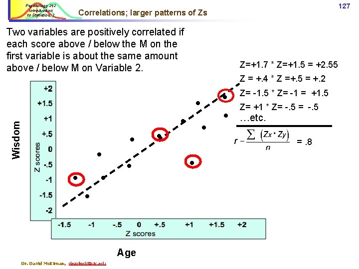
Psychology 242 Introduction to Statistics, 2 127 Correlations; larger patterns of Zs Two variables are positively correlated if each score above / below the M on the first variable is about the same amount above / below M on Variable 2. Z=+1. 7 * Z=+1. 5 = +2. 55 Z = +. 4 * Z =+. 5 = +. 2 Wisdom Age Dr. David Mc. Kirnan, davidmck@uic. edu Z= -1. 5 * Z= -1 = +1. 5 Z= +1 * Z= -. 5 …etc. =. 8

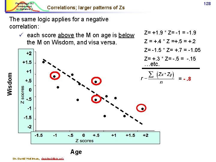
Psychology 242 Introduction to Statistics, 2 128 Correlations; larger patterns of Zs The same logic applies for a negative correlation: ü each score above the M on age is below the M on Wisdom, and visa versa. Z= +1. 9 * Z= -1. 9 Z = +. 4 * Z =+. 5 = +. 2 Z= -1. 5 * Z= +. 7 = -1. 05 Z= +. 3 * Z= -. 5 = -. 15 Wisdom …etc. = -. 8 Age Dr. David Mc. Kirnan, davidmck@uic. edu

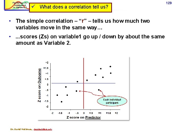
Psychology 242 Introduction to Statistics, 2 ü What does a correlation tell us? • The simple correlation – “r” – tells us how much two variables move in the same way… • . . . scores (Zs) on variable 1 go up / down by about the same amount as Variable 2. Dr. David Mc. Kirnan, davidmck@uic. edu 129

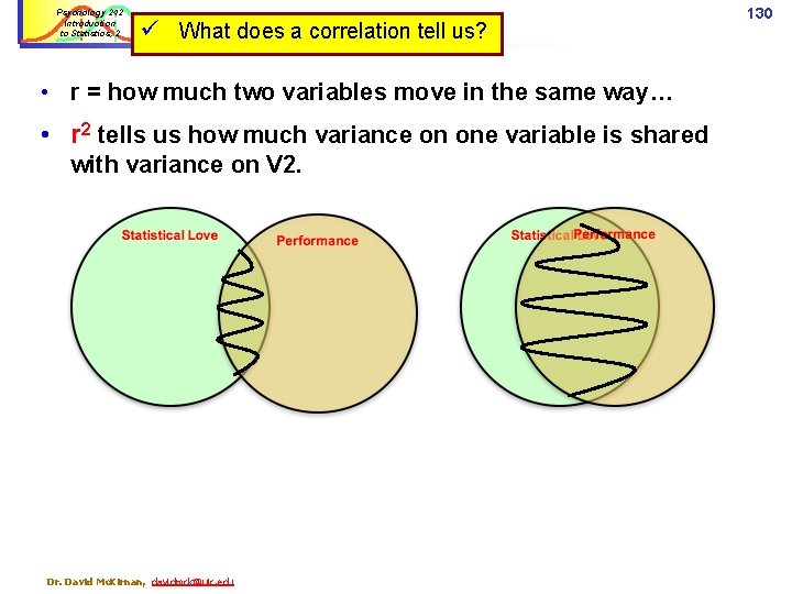
Psychology 242 Introduction to Statistics, 2 ü What does a correlation tell us? • r = how much two variables move in the same way… • r 2 tells us how much variance on one variable is shared with variance on V 2. Dr. David Mc. Kirnan, davidmck@uic. edu 130

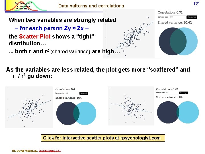
Psychology 242 Introduction to Statistics, 2 Data patterns and correlations When two variables are strongly related – for each person Zy ≈ Zx – the Scatter Plot shows a “tight” distribution…. . . both r and r 2 (shared variance) are high… As the variables are less related, the plot gets more “scattered” and r / r 2 go down: Click for interactive scatter plots at rpsychologist. com Dr. David Mc. Kirnan, davidmck@uic. edu 131

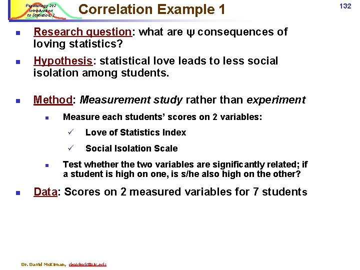
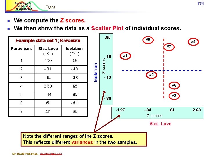
Correlation Example 1 Psychology 242 Introduction to Statistics, 2 n n n Research question: what are ψ consequences of loving statistics? Hypothesis: statistical love leads to less social isolation among students. Method: Measurement study rather than experiment n n n Measure each students’ scores on 2 variables: ü Love of Statistics Index ü Social Isolation Scale Test whether the two variables are significantly related; if a student is high on one, is s/he also high on the other? Data: Scores on 2 measured variables for 7 students Dr. David Mc. Kirnan, davidmck@uic. edu 132

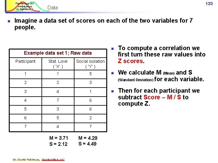
Psychology 242 Introduction to Statistics, 2 n 133 Data Imagine a data set of scores on each of the two variables for 7 people. Example data set 1; Raw data Participant Stat. Love ( ‘X’ ) Social isolation ( ‘Y’ ) 1 1 5 2 2 3 3 4 1 4 7 6 5 3 6 6 5 2 7 4 7 M = 3. 71 S = 2. 12 Dr. David Mc. Kirnan, davidmck@uic. edu M = 4. 29 S = 4. 49 n n n To compute a correlation we first turn these raw values into Z scores. We calculate M (Mean) and S (Standard Deviation) for each variable. Then for each participant we subtract Score – M / S to compute Z.

Psychology 242 Introduction to Statistics, 2 . 65 Example data set 1; Raw Z Scores data Participant Stat. Love ( ‘X’ ) Isolation ( ‘Y’ ) 1 -1. 27 1 . 16 5 2 -. 81 2 -. 13 3 3 . 14 4 -. 86 1 4 2. 03 7 . 65 6 5 -. 34 3 . 65 6 6 . 61 5 -. 51 2 7 . 34 4 . 60 7 #5 #4 #7 . 16 #1 Z scores n We compute the Z scores. We then show the data as a Scatter Plot of individual scores. Isolation n 134 Data #2 -. 13 #6 #3 -. 86 -1. 27 -. 34 Z scores . 61 Stat. Love Note the different ranges of the Z scores. This reflects different variances in the two samples. Dr. David Mc. Kirnan, davidmck@uic. edu 2. 03

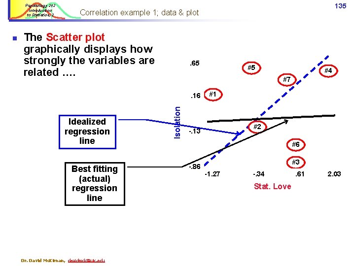
Psychology 242 Introduction to Statistics, 2 The Scatter plot graphically displays how strongly the variables are related …. . 65 . 16 Idealized regression line Best fitting (actual) regression line Dr. David Mc. Kirnan, davidmck@uic. edu #5 #4 #7 Isolation n 135 Correlation example 1; data & plot #1 #2 -. 13 #6 -. 86 #3 -1. 27 -. 34 Z scores Stat. Love . 61 2. 03

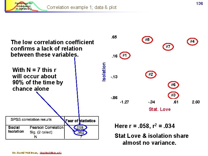
Psychology 242 Introduction to Statistics, 2 136 Correlation example 1; data & plot . 65 The low correlation coefficient confirms a lack of relation between these variables. #4 #7 . 16 Isolation With N = 7 this r will occur about 90% of the time by chance alone #5 #1 #2 -. 13 #6 -. 86 #3 -1. 27 -. 34 . 61 Stat. Love Here r =. 058, r 2 =. 034 Stat Love & isolation share almost no variance. Dr. David Mc. Kirnan, davidmck@uic. edu 2. 03

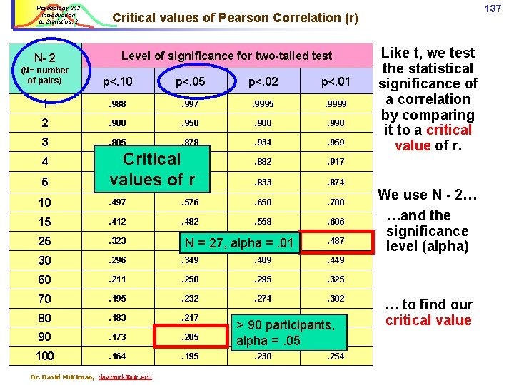
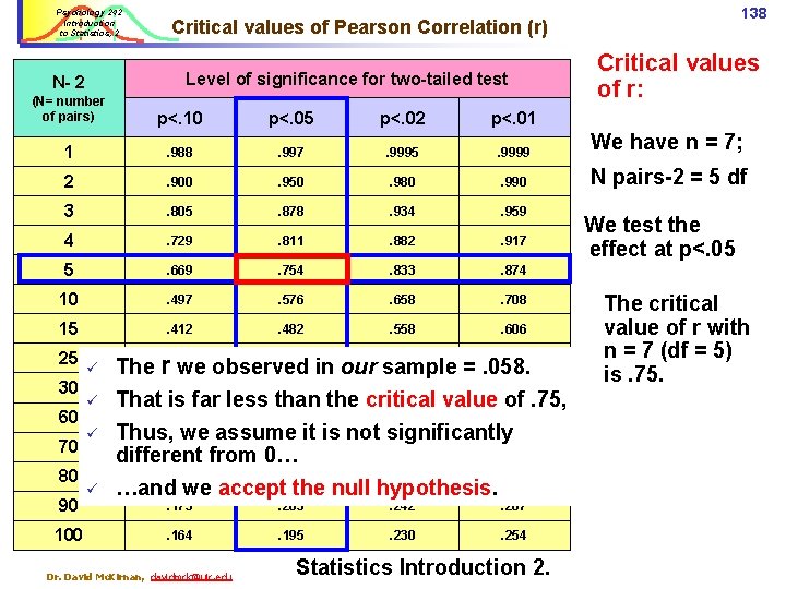
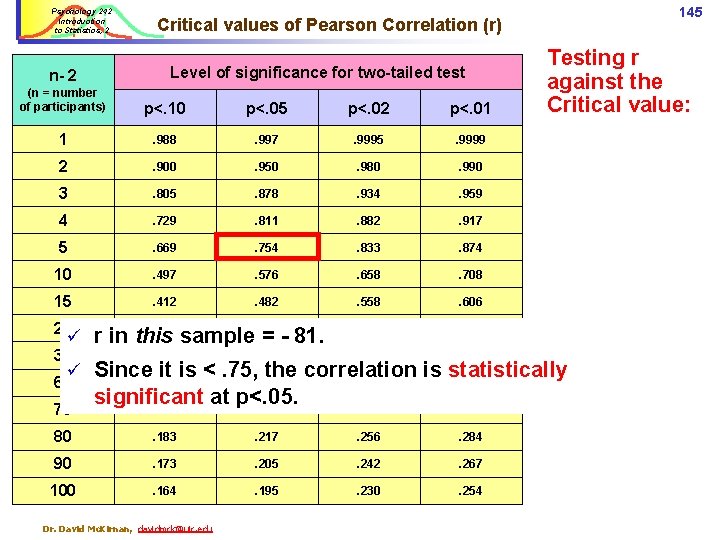
Psychology 242 Introduction to Statistics, 2 N- 2 Level of significance for two-tailed test (N= number of pairs) p<. 10 p<. 05 p<. 02 p<. 01 1 . 988 . 997 . 9995 . 9999 2 . 900 . 950 . 980 . 990 3 . 805 . 878 . 934 . 959 . 882 . 917 . 833 . 874 4 5 137 Critical values of Pearson Correlation (r) Critical. 811. 669 values of. 754 r. 729 10 . 497 . 576 . 658 . 708 15 . 412 . 482 . 558 . 606 25 . 323 . 381 N= 30 . 296 . 349 . 409 . 449 60 . 211 . 250 . 295 . 325 70 . 195 . 232 . 274 . 302 80 . 183 . 217 . 256 . 284 90 . 173 . 205 100 . 164 . 195 . 230 . 254 Dr. David Mc. Kirnan, davidmck@uic. edu . 445 27, alpha =. 01 . 487 > 90 participants, . 242. 267 alpha =. 05 Like t, we test the statistical significance of a correlation by comparing it to a critical value of r. We use N - 2… …and the significance level (alpha) … to find our critical value

Psychology 242 Introduction to Statistics, 2 Level of significance for two-tailed test N- 2 138 Critical values of Pearson Correlation (r) Critical values of r: (N= number of pairs) p<. 10 p<. 05 p<. 02 p<. 01 1 . 988 . 997 . 9995 . 9999 We have n = 7; 2 . 900 . 950 . 980 . 990 N pairs-2 = 5 df 3 . 805 . 878 . 934 . 959 4 . 729 . 811 . 882 . 917 5 . 669 . 754 . 833 . 874 10 . 497 . 576 . 658 . 708 15 . 412 . 482 . 558 . 606 25 30 60 70 80 90 100 ü ü . 381. 445. 487 The r. 323 we observed in our sample =. 058. . 296 . 349 . 409 . 449 . 173 . 205 . 242 . 267 . 164 . 195 . 230 . 254 That is far less than the critical value of. 75, . 211. 250. 295. 325 Thus, we assume it is not significantly. 195. 232. 274. 302 different from 0…. 183. 217. 256. 284 …and we accept the null hypothesis. Dr. David Mc. Kirnan, davidmck@uic. edu Statistics Introduction 2. We test the effect at p<. 05 The critical value of r with n = 7 (df = 5) is. 75.

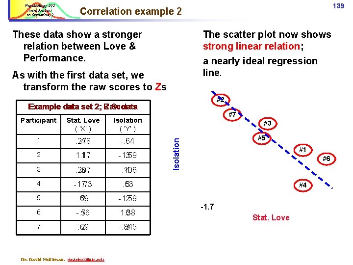
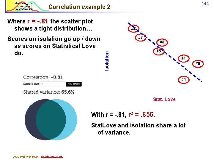
Psychology 242 Introduction to Statistics, 2 139 Correlation example 2 These data show a stronger relation between Love & Performance. The scatter plot now shows strong linear relation; a nearly ideal regression line. As with the first data set, we transform the raw scores to Zs #2 Example data set 2; Raw Z Scores data Stat. Love ( ‘X’ ) Isolation ( ‘Y’ ) 1 . 278 4 -. 64 5 2 1. 17 1 -1. 59 3 3 . 207 3 -. 106 4 4 -1. 73 7 . 63 5 5 . 69 2 -1. 59 2 6 -. 76 5 1. 38 6 7 . 69 2 -. 845 3 Dr. David Mc. Kirnan, davidmck@uic. edu #7 #3 #5 Isolation Participant #1 #6 #4 -1. 7 Stat. Love

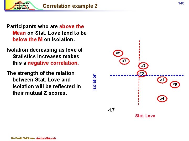
Psychology 242 Introduction to Statistics, 2 140 Correlation example 2 Participants who are above the Mean on Stat. Love tend to be below the M on Isolation decreasing as love of Statistics increases makes this a negative correlation. #7 #3 #5 Isolation The strength of the relation between Stat. Love and Isolation will be reflected in their mutual Z scores. #2 #1 #6 #4 -1. 7 Stat. Love Dr. David Mc. Kirnan, davidmck@uic. edu

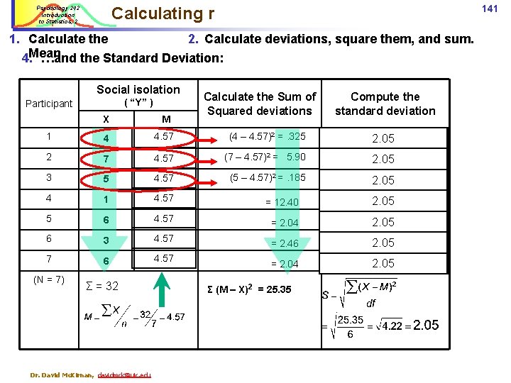
141 Calculating r Psychology 242 Introduction to Statistics, 2 1. Calculate the 2. Calculate deviations, square them, and sum. 4. Mean. …and the Standard Deviation: Social isolation ( “Y” ) Participant Calculate the Sum of Squared deviations Compute the standard deviation X M 1 4 4. 57 (4 – 4. 57)2 =. 325 2. 05 2 7 4. 57 (7 – 4. 57)2 = 5. 90 2. 05 3 5 4. 57 (5 – 4. 57)2 =. 185 2. 05 4 1 4. 57 = 12. 40 2. 05 5 6 4. 57 = 2. 04 2. 05 6 3 4. 57 = 2. 46 2. 05 7 6 4. 57 = 2. 04 2. 05 (N = 7) Σ = 32 Dr. David Mc. Kirnan, davidmck@uic. edu Σ (M – X)2 = 25. 35

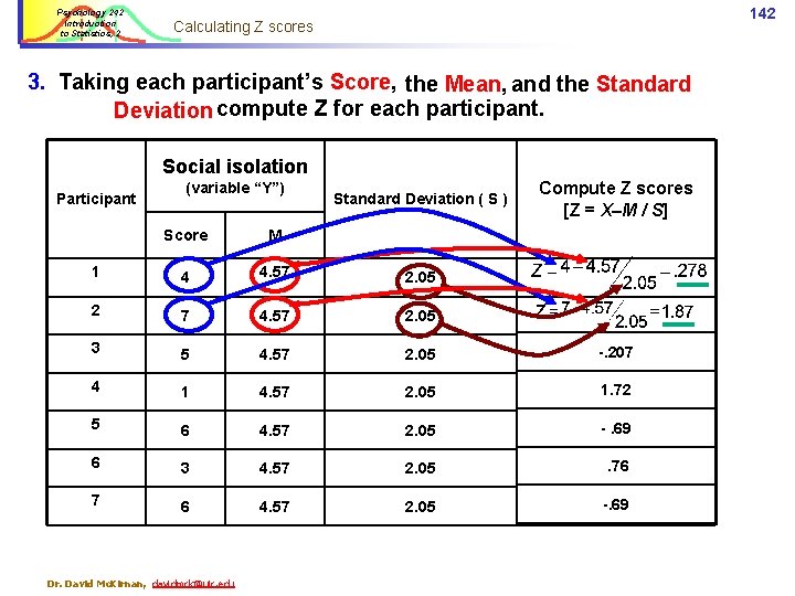
Psychology 242 Introduction to Statistics, 2 142 Calculating Z scores 3. Taking each participant’s Score, the Mean, and the Standard Deviation compute Z for each participant. Social isolation Participant (variable “Y”) Standard Deviation ( S ) Compute Z scores [Z = X–M / S] Score M 1 4 4. 57 2. 05 2 7 4. 57 2. 05 3 5 4. 57 2. 05 -. 207 4 1 4. 57 2. 05 1. 72 5 6 4. 57 2. 05 -. 69 6 3 4. 57 2. 05 . 76 7 6 4. 57 2. 05 -. 69 Dr. David Mc. Kirnan, davidmck@uic. edu

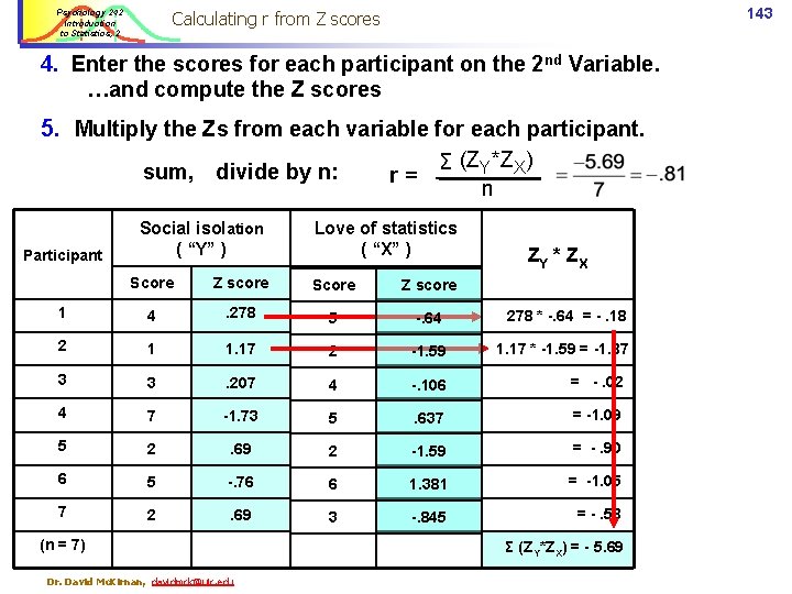
143 Calculating r from Z scores Psychology 242 Introduction to Statistics, 2 4. Enter the scores for each participant on the 2 nd Variable. …and compute the Z scores 5. Multiply the Zs from each variable for each participant. sum, divide by n: Participant Social isolation ( “Y” ) Σ (ZY*ZX) r= n Love of statistics ( “X” ) ZY * Z X Score Z score 1 4 . 278 5 -. 64 278 * -. 64 = -. 18 2 1 1. 17 2 -1. 59 1. 17 * -1. 59 = -1. 87 3 3 . 207 4 -. 106 = -. 02 4 7 -1. 73 5 . 637 = -1. 09 5 2 . 69 2 -1. 59 = -. 90 6 5 -. 76 6 1. 381 = -1. 05 7 2 . 69 3 -. 845 = -. 58 (n = 7) Dr. David Mc. Kirnan, davidmck@uic. edu Σ (ZY*ZX) = - 5. 69

Psychology 242 Introduction to Statistics, 2 144 Correlation example 2 Where r = -. 81 the scatter plot shows a tight distribution… #7 #3 #5 Isolation Scores on isolation go up / down as scores on Statistical Love do. #2 #1 #6 #4 Stat. Love With r = -. 81, r 2 =. 656. Stat. Love and isolation share a lot of variance. Dr. David Mc. Kirnan, davidmck@uic. edu

Psychology 242 Introduction to Statistics, 2 Level of significance for two-tailed test n- 2 (n = number of participants) p<. 10 p<. 05 p<. 02 p<. 01 1 . 988 . 997 . 9995 . 9999 2 . 900 . 950 . 980 . 990 3 . 805 . 878 . 934 . 959 4 . 729 . 811 . 882 . 917 5 . 669 . 754 . 833 . 874 10 . 497 . 576 . 658 . 708 15 . 412 . 482 . 558 . 606 . 445 . 487 25 ü 30 . 323 r in this sample. 381 = - 81. . 296 . 349 . 409 . 449 80 . 183 . 217 . 256 . 284 90 . 173 . 205 . 242 . 267 100 . 164 . 195 . 230 . 254 ü 60 70 145 Critical values of Pearson Correlation (r) Testing r against the Critical value: Since. 211 it is <. 75, . 250 the correlation is statistically. 295. 325 significant at p<. 05. . 195. 232. 274. 302 Dr. David Mc. Kirnan, davidmck@uic. edu

Psychology 242 Introduction to Statistics, 2 146 Summary: Statistical tests t-test: Compare one group to another Experimental v. control (Experiment) Men v. women, etc. (Measurement) n n n Calculate M for each group, compare them to determine how much variance is due to differences between groups. Calculate standard error to determine how much variance is due to individual differences within each group. Calculate the critical ratio (t): Difference between groups standard error of M Dr. David Mc. Kirnan, davidmck@uic. edu

Psychology 242 Introduction to Statistics, 2 Statistics summary: correlation Pearson Correlation (r): how similar is the variance between two variables within a sample. n Are people above or below the mean on one variable similarly above or below M on the second variable? r = the product of each participant’s Z score for two variables / n: r 2 measures how much variance is shared between two variables. Dr. David Mc. Kirnan, davidmck@uic. edu 147

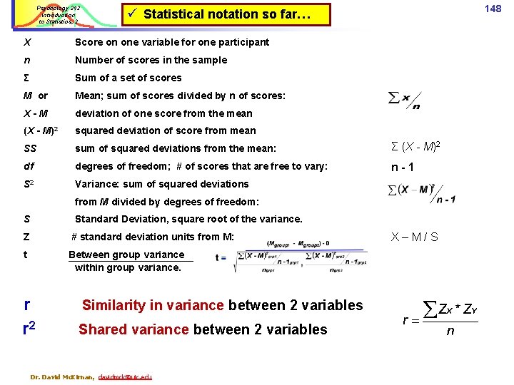
Psychology 242 Introduction to Statistics, 2 148 ü Statistical notation so far… X Score on one variable for one participant n Number of scores in the sample Σ Sum of a set of scores M or Mean; sum of scores divided by n of scores: X-M deviation of one score from the mean (X - M)2 squared deviation of score from mean SS sum of squared deviations from the mean: Σ (X - M)2 df degrees of freedom; # of scores that are free to vary: n-1 S 2 Variance: sum of squared deviations from M divided by degrees of freedom: S Standard Deviation, square root of the variance. Z # standard deviation units from M: t Between group variance within group variance. r r 2 Similarity in variance between 2 variables Shared variance between 2 variables Dr. David Mc. Kirnan, davidmck@uic. edu X–M/S

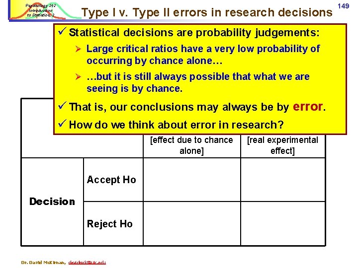
Psychology 242 Introduction to Statistics, 2 Type I v. Type II errors in research decisions ü Statistical decisions are probability judgements: Ø Large critical ratios have a very low probability of occurring by chance alone… Ø …but it is still always possible that we are seeing is by chance. ü That is, our conclusions may always be by error. “Reality” ü How do we think about error in research? Ho true Ho false [effect due to chance alone] Accept Ho Decision Reject Ho Dr. David Mc. Kirnan, davidmck@uic. edu [real experimental effect] 149

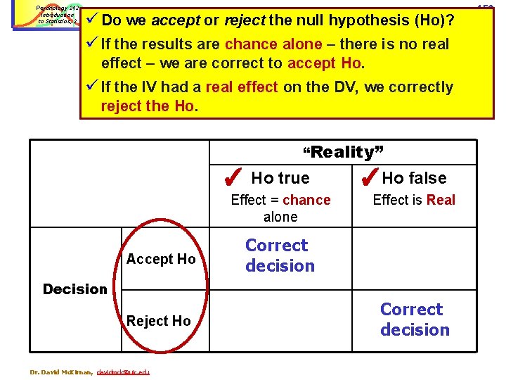
Psychology 242 Introduction to Statistics, 2 ü Do we accept or reject the null hypothesis (Ho)? ü If the results are chance alone – there is no real Type I v. Type II errors effect – we are correct to accept Ho. ü If the IV had a real effect on the DV, we correctly reject the Ho. “Reality” ✓ Ho true Effect = chance alone Accept Ho Decision Reject Ho Dr. David Mc. Kirnan, davidmck@uic. edu ✓Ho false Effect is Real Correct decision 150

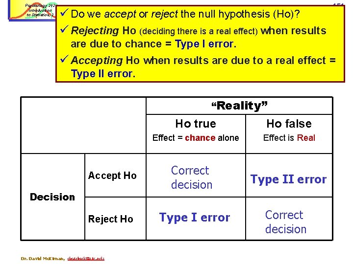
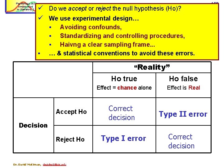
Psychology 242 Introduction to Statistics, 2 ü Do we accept or reject the null hypothesis (Ho)? ü Rejecting Ho (deciding there is a real effect) when results Type I v. Type II errors 151 are due to chance = Type I error. ü Accepting Ho when results are due to a real effect = Type II error. “Reality” Ho true Ho false Effect = chance alone Effect is Real Accept Ho Correct decision Type II error Reject Ho Type I error Correct decision Dr. David Mc. Kirnan, davidmck@uic. edu

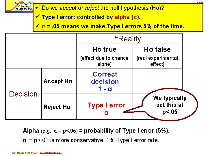
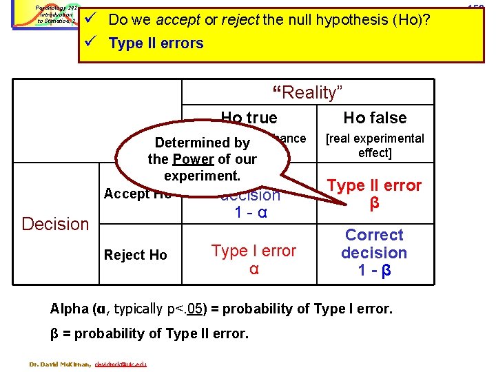
Psychology 242 Introduction to Statistics, 2 Inferring ‘reality’: Type I & Type II errors; ü Do we accept or reject the null hypothesis (Ho)? ü Type I error: controlled by alpha (α). ü α = , 05 means we make Type I errors 5% of the time. “Reality” Accept Ho Decision Reject Ho Ho true Ho false [effect due to chance alone] [real experimental effect] Correct decision 1 -α Type I error α We typically set this at p<. 05 Alpha (e. g. , α = p<. 05) = probability of Type I error (5%). α = p<. 01 is more conservative: 1% Type I error rate. Dr. David Mc. Kirnan, davidmck@uic. edu 152

Psychology 242 Introduction to Statistics, 2 153 Statistical Decision Making: Errors Type I error; Reject the null hypothesis [Ho] when it is actually true: n Accept as ‘real’ an effect that is due to chance only § Type I error rate is determined by Alpha (. 10 . 05 . 01 . 001…) § As we choose a less stringent alpha level, critical values get lower. § This makes it easier to commit a Type I error. § Type I is the “worst” error; our statistical conventions are designed to prevent these. Dr. David Mc. Kirnan, davidmck@uic. edu

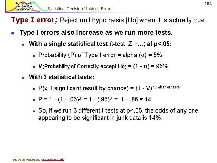
Psychology 242 Introduction to Statistics, 2 154 Statistical Decision Making: Errors Type I error; Reject null hypothesis [Ho] when it is actually true: n Type I errors also increase as we run more tests. n n With a single statistical test (t-test, Z, r…) at p<. 05: n Probability (P) of Type I error = alpha (α) = 5%. n V(Probability of Correctly accept Ho) = (1 - α) = 95%. With 3 statistical tests: n P(≥ 1 significant result by chance) = (1 - V)number of tests n P = 1 - (1 -. 05)3 = 1 - (. 95)3 = 1 -. 86 ≈. 14 n So, if we run 3 different t-tests at p<. 05, the odds of any one appearing to be significant in junk data is 14%. Dr. David Mc. Kirnan, davidmck@uic. edu

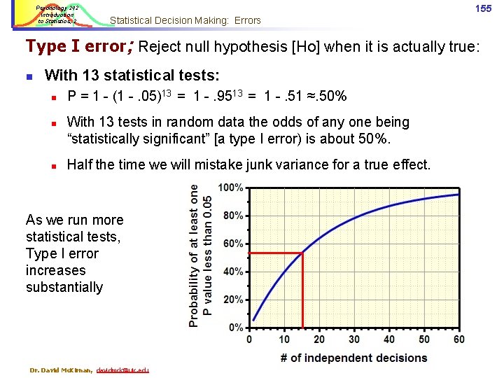
Psychology 242 Introduction to Statistics, 2 155 Statistical Decision Making: Errors Type I error; Reject null hypothesis [Ho] when it is actually true: n With 13 statistical tests: n n n P = 1 - (1 -. 05)13 = 1 -. 9513 = 1 -. 51 ≈. 50% With 13 tests in random data the odds of any one being “statistically significant” [a type I error) is about 50%. Half the time we will mistake junk variance for a true effect. As we run more statistical tests, Type I error increases substantially Dr. David Mc. Kirnan, davidmck@uic. edu

Psychology 242 Introduction to Statistics, 2 Inferring ‘reality’: Type I & Type II errors; ü Do we accept or reject the null hypothesis (Ho)? ü Type II errors “Reality” Ho true [effect due Determined by to chance the Power of alone] our experiment. Correct Accept Ho decision 1 -α Decision Reject Ho Type I error α Ho false [real experimental effect] Type II error β Correct decision 1 -β Alpha (α, typically p<. 05) = probability of Type I error. β = probability of Type II error. David Mc. Kirnan, davidmck@uic. edu 156

Psychology 242 Introduction to Statistics, 2 157 Statistical Decision Making: Errors Type II error; Accept Ho when it is actually false; n Type II rate most strongly affected by statistical power. Central Limit Theorem: Smaller samples n n n Assume more variance More conservative critical value Smaller samples have more stringent critical values… So they have less ‘power’ to detect a significant effect. In small “underpowered” samples it is difficult for even strong effects to come out statistically significant. Dr. David Mc. Kirnan, davidmck@uic. edu

Psychology 242 Introduction to Statistics, 2 ü Do we accept or reject the null hypothesis (Ho)? ü We use experimental design… Type I v. Type II errors Avoiding confounds, § Standardizing and controlling procedures, § Haivng a clear sampling frame. . . … & statistical conventions to avoid these errors. § § “Reality” Ho true Ho false Effect = chance alone Effect is Real Accept Ho Correct decision Type II error Reject Ho Type I error Correct decision Dr. David Mc. Kirnan, davidmck@uic. edu 158

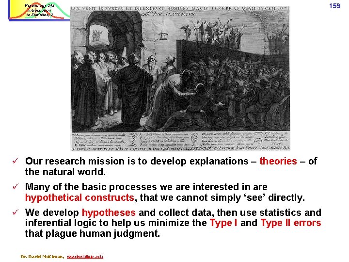
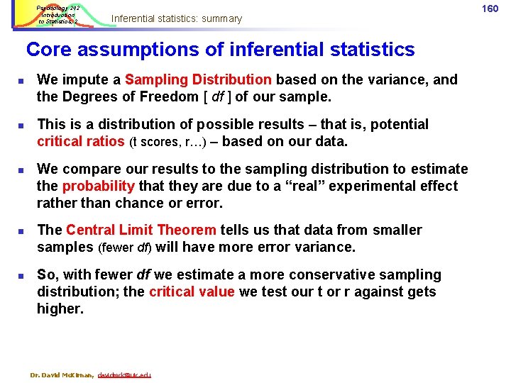
159 Psychology 242 Introduction to Statistics, 2 Inferential statistics: summary ü Our research mission is to develop explanations – theories – of the natural world. ü Many of the basic processes we are interested in are hypothetical constructs, that we cannot simply ‘see’ directly. ü We develop hypotheses and collect data, then use statistics and inferential logic to help us minimize the Type I and Type II errors that plague human judgment. Dr. David Mc. Kirnan, davidmck@uic. edu

Psychology 242 Introduction to Statistics, 2 Inferential statistics: summary Core assumptions of inferential statistics n n n We impute a Sampling Distribution based on the variance, and the Degrees of Freedom [ df ] of our sample. This is a distribution of possible results – that is, potential critical ratios (t scores, r…) – based on our data. We compare our results to the sampling distribution to estimate the probability that they are due to a “real” experimental effect rather than chance or error. The Central Limit Theorem tells us that data from smaller samples (fewer df) will have more error variance. So, with fewer df we estimate a more conservative sampling distribution; the critical value we test our t or r against gets higher. Dr. David Mc. Kirnan, davidmck@uic. edu 160

Psychology 242 Introduction to Statistics, 2 n n Plato’s cave and the estimation of “reality” Inferences about our observations: n n n Inferential statistics: summary, Key terms Deductive v. Inductive link of theory / hypothetical constructs & data Generalizing results beyond the experiment Critical ratio (you will be asked to produce and describe this). Variance, variability in different distributions Degrees of Freedom [df] t-test, between versus within –group variance Sampling distribution, M of the sampling distribution Alpha (α), critical value t table, general logic of calculating a t-test “Shared variance”, positive / negative correlation General logic of calculating a correlation (mutual Z scores). Null hypothesis, Type I & Type II errors. Dr. David Mc. Kirnan, davidmck@uic. edu 161