ET 242 Circuit Analysis II Parallel Resonance Electrical

ET 242 Circuit Analysis II Parallel Resonance Electrical and Telecommunication Engineering Technology Professor Jang

Acknowledgement I want to express my gratitude to Prentice Hall giving me the permission to use instructor’s material for developing this module. I would like to thank the Department of Electrical and Telecommunications Engineering Technology of NYCCT for giving me support to commence and complete this module. I hope this module is helpful to enhance our students’ academic performance.

OUTLINES Ø Introduction to Parallel Resonance Ø Parallel Resonance Circuit Ø Unity Power Factor (fp) Ø Selectivity Curve Ø Effect of QL ≥ 10 Ø Examples Key Words: Resonance, Unity Power Factor, Selective Curve, Quality Factor ET 242 Circuit Analysis II – Parallel Resonance Boylestad 2

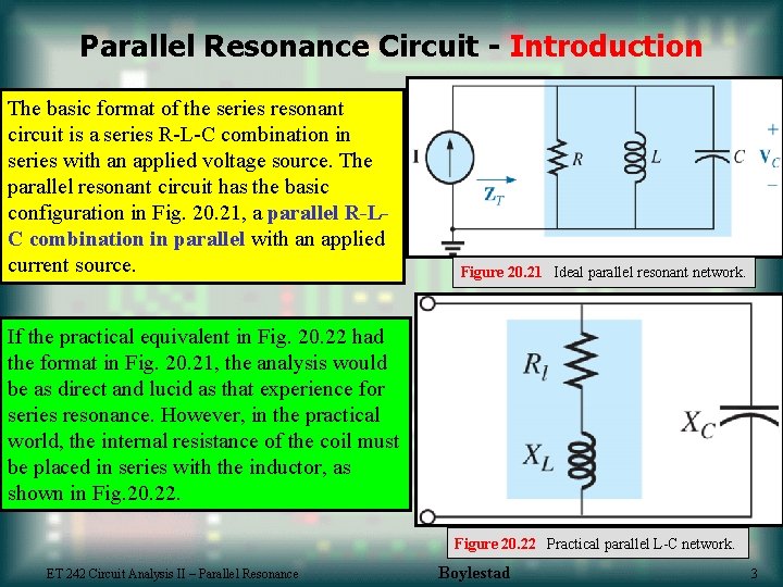
Parallel Resonance Circuit - Introduction The basic format of the series resonant circuit is a series R-L-C combination in series with an applied voltage source. The parallel resonant circuit has the basic configuration in Fig. 20. 21, a parallel R-LC combination in parallel with an applied current source. Figure 20. 21 Ideal parallel resonant network. If the practical equivalent in Fig. 20. 22 had the format in Fig. 20. 21, the analysis would be as direct and lucid as that experience for series resonance. However, in the practical world, the internal resistance of the coil must be placed in series with the inductor, as shown in Fig. 20. 22. Figure 20. 22 Practical parallel L-C network. ET 242 Circuit Analysis II – Parallel Resonance Boylestad 3

The first effort is to find a parallel network equivalent for the series R-L branch in Fig. 20. 22 using the technique in earlier section. That is Figure 20. 23 Equivalent parallel network for a series R-L combination. Parallel Resonant Circuit – Unity Power Factor, fp Figure 20. 25 Substituting R = Rs//Rp for the network in Fig. 20. 24. ET 162 Circuit Analysis – Parallel Resonance Boylestad 4

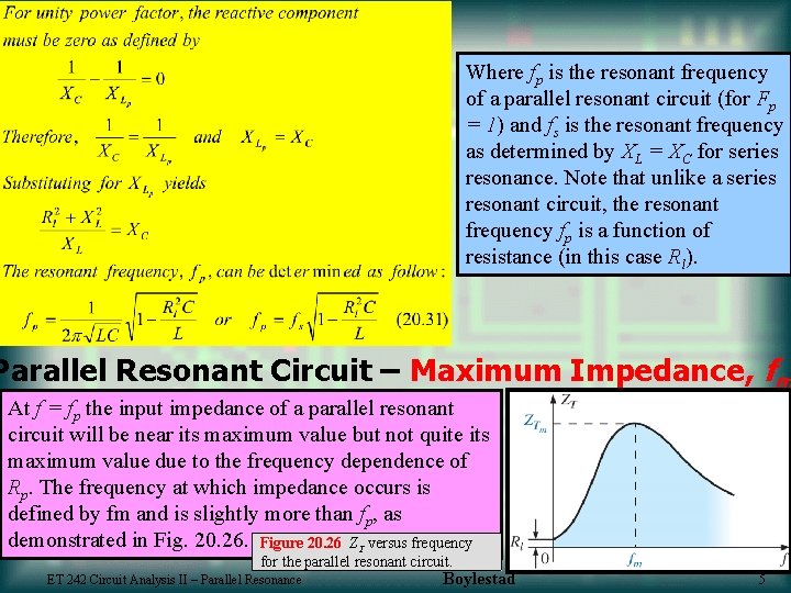
Where fp is the resonant frequency of a parallel resonant circuit (for Fp = 1) and fs is the resonant frequency as determined by XL = XC for series resonance. Note that unlike a series resonant circuit, the resonant frequency fp is a function of resistance (in this case Rl). Parallel Resonant Circuit – Maximum Impedance, fm At f = fp the input impedance of a parallel resonant circuit will be near its maximum value but not quite its maximum value due to the frequency dependence of Rp. The frequency at which impedance occurs is defined by fm and is slightly more than fp, as demonstrated in Fig. 20. 26. Figure 20. 26 ZT versus frequency for the parallel resonant circuit. ET 242 Circuit Analysis II – Parallel Resonance Boylestad 5

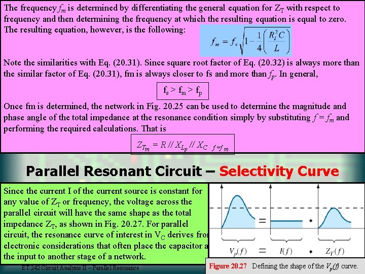
The frequency fm is determined by differentiating the general equation for ZT with respect to frequency and then determining the frequency at which the resulting equation is equal to zero. The resulting equation, however, is the following: Note the similarities with Eq. (20. 31). Since square root factor of Eq. (20. 32) is always more than the similar factor of Eq. (20. 31), fm is always closer to fs and more than fp. In general, fs > f m > fp Once fm is determined, the network in Fig. 20. 25 can be used to determine the magnitude and phase angle of the total impedance at the resonance condition simply by substituting f = fm and performing the required calculations. That is ZTm = R // XLp // XC f =f m Parallel Resonant Circuit – Selectivity Curve Since the current I of the current source is constant for any value of ZT or frequency, the voltage across the parallel circuit will have the same shape as the total impedance ZT, as shown in Fig. 20. 27. For parallel circuit, the resonance curve of interest in VC derives from electronic considerations that often place the capacitor at the input to another stage of a network. ET 242 Circuit Analysis II – Parallel Resonance Figure 20. 27 Defining the shape of the Vp(f) curve. Boylestad 6

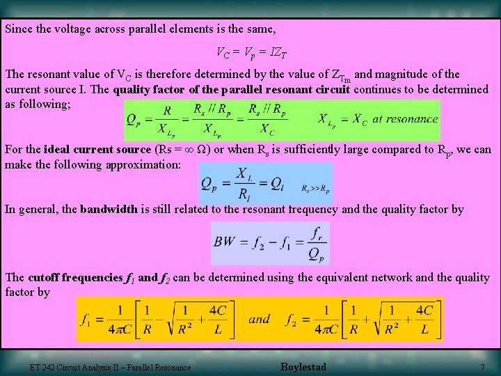
Since the voltage across parallel elements is the same, VC = Vp = IZT The resonant value of VC is therefore determined by the value of ZTm and magnitude of the current source I. The quality factor of the parallel resonant circuit continues to be determined as following; For the ideal current source (Rs = ∞ Ω) or when Rs is sufficiently large compared to Rp, we can make the following approximation: In general, the bandwidth is still related to the resonant frequency and the quality factor by The cutoff frequencies f 1 and f 2 can be determined using the equivalent network and the quality factor by ET 242 Circuit Analysis II – Parallel Resonance Boylestad 7

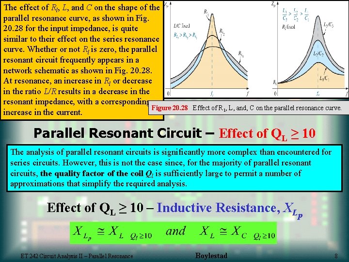
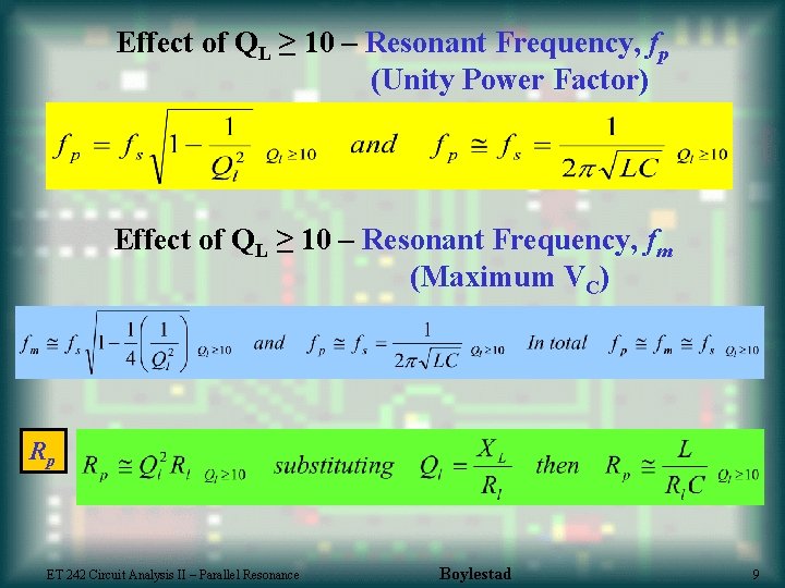
The effect of Rl, L, and C on the shape of the parallel resonance curve, as shown in Fig. 20. 28 for the input impedance, is quite similar to their effect on the series resonance curve. Whether or not Rl is zero, the parallel resonant circuit frequently appears in a network schematic as shown in Fig. 20. 28. At resonance, an increase in Rl or decrease in the ratio L/R results in a decrease in the resonant impedance, with a corresponding Figure 20. 28 increase in the current. Effect of R 1, L, and, C on the parallel resonance curve. Parallel Resonant Circuit – Effect of QL ≥ 10 The analysis of parallel resonant circuits is significantly more complex than encountered for series circuits. However, this is not the case since, for the majority of parallel resonant circuits, the quality factor of the coil Ql is sufficiently large to permit a number of approximations that simplify the required analysis. Effect of QL ≥ 10 – Inductive Resistance, XLp ET 242 Circuit Analysis II – Parallel Resonance Boylestad 8

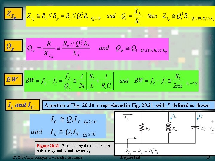
Effect of QL ≥ 10 – Resonant Frequency, fp (Unity Power Factor) Effect of QL ≥ 10 – Resonant Frequency, fm (Maximum VC) Rp ET 242 Circuit Analysis II – Parallel Resonance Boylestad 9

Z Tp Qp BW IL and IC A portion of Fig. 20. 30 is reproduced in Fig. 20. 31, with IT defined as shown Figure 20. 31 Establishing the relationship between IC and IL and current IT. ET 242 Circuit Analysis II – Parallel Resonance Boylestad 10

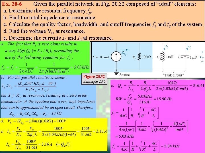
Ex. 20 -6 Given the parallel network in Fig. 20. 32 composed of “ideal” elements: a. Determine the resonant frequency fp. b. Find the total impedance at resonance c. Calculate the quality factor, bandwidth, and cutoff frequencies f 1 and f 2 of the system. d. Find the voltage VC at resonance. e. Determine the currents IL and IC at resonance. Figure 20. 32 Example 20. 6. ET 242 Circuit Analysis II – Power for AC Circuits Boylestad 11

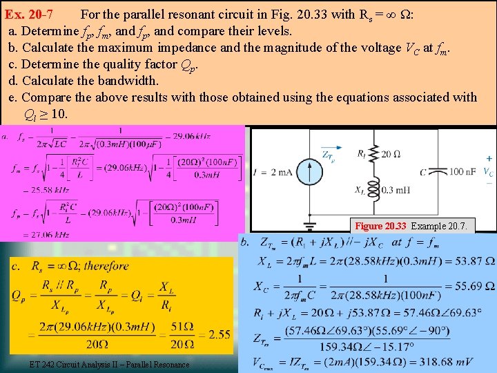
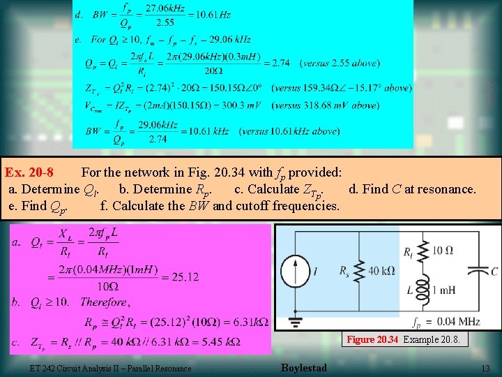
Ex. 20 -7 For the parallel resonant circuit in Fig. 20. 33 with Rs = ∞ Ω: a. Determine fp, fm, and fp, and compare their levels. b. Calculate the maximum impedance and the magnitude of the voltage VC at fm. c. Determine the quality factor Qp. d. Calculate the bandwidth. e. Compare the above results with those obtained using the equations associated with Ql ≥ 10. Figure 20. 33 Example 20. 7. ET 242 Circuit Analysis II – Parallel Resonance Boylestad 12

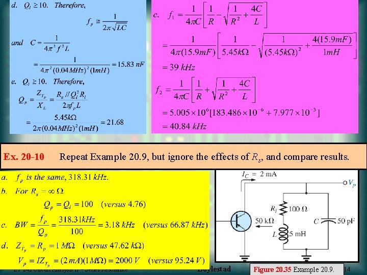
Ex. 20 -8 For the network in Fig. 20. 34 with fp provided: a. Determine Ql. b. Determine Rp. c. Calculate ZTp. d. Find C at resonance. e. Find Qp. f. Calculate the BW and cutoff frequencies. Figure 20. 34 Example 20. 8. ET 242 Circuit Analysis II – Parallel Resonance Boylestad 13

Ex. 20 -10 Repeat Example 20. 9, but ignore the effects of Rs, and compare results. ET 242 Circuit Analysis II – Series Resonance Boylestad Figure 20. 35 Example 20. 9. 14