Psychology 242 Introduction to Research 1 Statistics 2

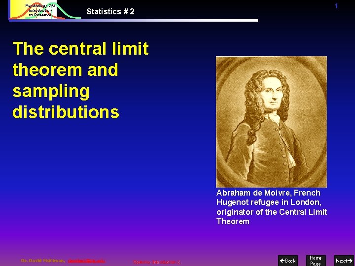
Psychology 242 Introduction to Research 1 Statistics # 2 The central limit theorem and sampling distributions Abraham de Moivre, French Hugenot refugee in London, originator of the Central Limit Theorem Dr. David Mc. Kirnan, davidmck@uic. edu Statistics Introduction 2. Back Home Page Next

Psychology 242 Introduction to Research 2 Central limit theorem The Central Limit Theorem Our evaluation of a t score for statistical significance depends on sample size: n n Larger samples yield more “normal”, tighter distributions (less error variance…). With smaller samples we use more conservative assumptions about the sampling distribution. Dr. David Mc. Kirnan, davidmck@uic. edu Statistics Introduction 2. Back Home Page Next

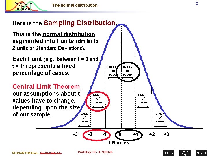
Psychology 242 Introduction to Research 3 The normal distribution Here is the Sampling Distribution. This is the normal distribution, segmented into t units (similar to Z units or Standard Deviations). Each t unit (e. g. , between t = 0 and t = 1) represents a fixed percentage of cases. 34. 13% of of cases Central Limit Theorem: our assumptions about t values have to change, depending upon the size 2. 25% of our sample. of 13. 59% of cases 2. 25% of cases -3 -2 -1 0 +1 +2 +3 t Scores Dr. David Mc. Kirnan, davidmck@uic. edu Psychology 242, Dr. Mc. Kirnan Back Home Page Next

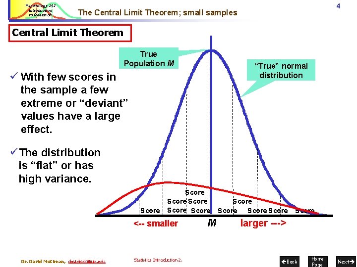
Psychology 242 Introduction to Research 4 The Central Limit Theorem; small samples Central Limit Theorem True Population M “True” normal distribution ü With few scores in the sample a few extreme or “deviant” values have a large effect. ü The distribution is “flat” or has high variance. Score Score <-- smaller Dr. David Mc. Kirnan, davidmck@uic. edu Statistics Introduction 2. M Score Score larger ---> Back Home Page Next

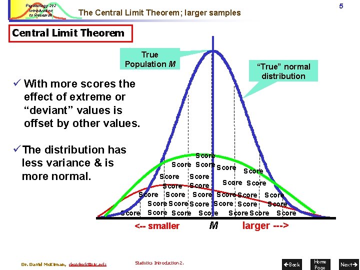
Psychology 242 Introduction to Research 5 The Central Limit Theorem; larger samples Central Limit Theorem True Population M “True” normal distribution ü With more scores the effect of extreme or “deviant” values is offset by other values. ü The distribution has less variance & is more normal. Score Score Score Score Score Score Score Score <-- smaller Dr. David Mc. Kirnan, davidmck@uic. edu Statistics Introduction 2. M larger ---> Back Home Page Next

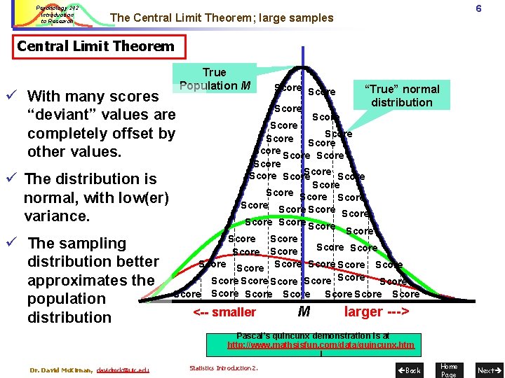
Psychology 242 Introduction to Research 6 The Central Limit Theorem; large samples Central Limit Theorem ü With many scores “deviant” values are completely offset by other values. ü The distribution is normal, with low(er) variance. ü The sampling distribution better approximates the population distribution True Population M Score “True” normal distribution Score Score Score Score Score Score Score Score Score Score Score Score <-- smaller Score M Score larger ---> Pascal’s quincunx demonstration is at http: //www. mathsisfun. com/data/quincunx. htm l Dr. David Mc. Kirnan, davidmck@uic. edu Statistics Introduction 2. Back Home Page Next

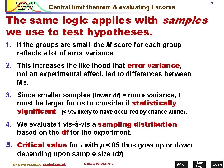
Psychology 242 Introduction to Research 7 Central limit theorem & evaluating t scores The same logic applies with samples we use to test hypotheses. 1. If the groups are small, the M score for each group reflects a lot of error variance. 2. This increases the likelihood that error variance, not an experimental effect, led to differences between Ms. 3. Since smaller samples (lower df) = more variance, t must be larger for us to consider it statistically significant (< 5% likely to have occurred by chance alone). 4. We evaluate t vis-à-vis a sampling distribution based on the df for the experiment. 5. Critical value for t with p <. 05 thus goes up or down depending upon sample size (df) Dr. David Mc. Kirnan, davidmck@uic. edu Statistics Introduction 2. Back Home Page Next

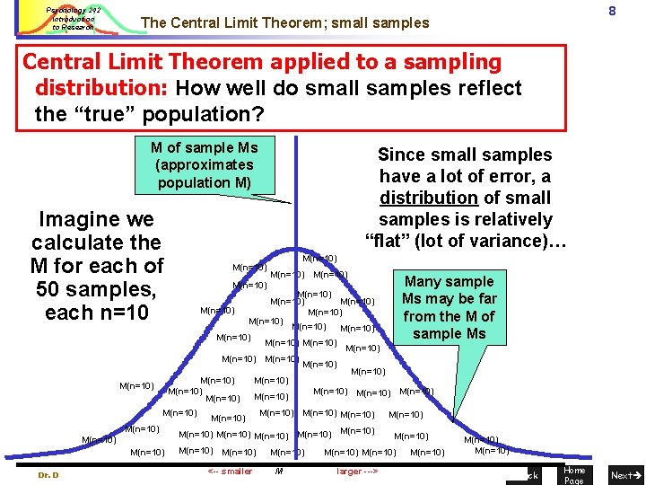
Psychology 242 Introduction to Research 8 The Central Limit Theorem; small samples Central Limit Theorem applied to a sampling distribution: How well do small samples reflect the “true” population? M of sample Ms (approximates population M) Imagine we calculate the M for each of 50 samples, each n=10 M(n=10) M(n=10) Many sample Ms may be far from the M of sample Ms M(n=10) M(n=10) M(n=10) M(n=10) M(n=10) M(n=10) M(n=10) Since small samples have a lot of error, a distribution of small samples is relatively “flat” (lot of variance)… M(n=10) M(n=10) M(n=10) Dr. David Mc. Kirnan, davidmck@uic. edu M(n=10) <-- smaller M 2. Statistics Introduction M(n=10) larger ---> M(n=10) Back Home Page Next

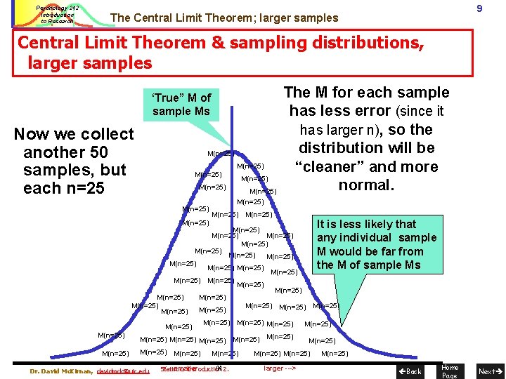
Psychology 242 Introduction to Research 9 The Central Limit Theorem; larger samples Central Limit Theorem & sampling distributions, larger samples ‘True” M of sample Ms Now we collect another 50 samples, but each n=25 M(n=25) M(n=25) The M for each sample has less error (since it has larger n), so the distribution will be “cleaner” and more normal. M(n=25) It is less likely that any individual sample M would be far from the M of sample Ms M(n=25) M(n=25) M(n=25) M(n=25) M(n=25) M(n=25) M(n=25) M(n=25) M(n=25) M(n=25) Dr. David Mc. Kirnan, davidmck@uic. edu M(n=25) <-- smaller M 2. Statistics Introduction M(n=25) larger ---> M(n=25) Back Home Page Next

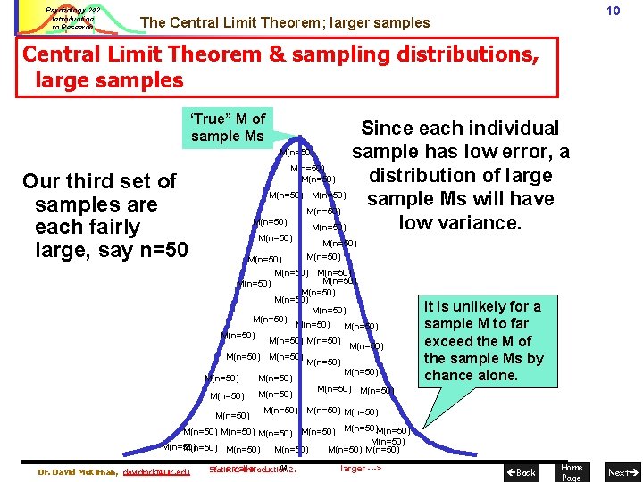
Psychology 242 Introduction to Research 10 The Central Limit Theorem; larger samples Central Limit Theorem & sampling distributions, large samples ‘True” M of sample Ms Our third set of samples are each fairly large, say n=50 Since each individual M(n=50) sample has low error, a M(n=50) distribution of large M(n=50) sample Ms will have M(n=50) low variance. M(n=50) M(n=50) M(n=50) M(n=50) M(n=50) M(n=50) M(n=50) M(n=50) It is unlikely for a sample M to far exceed the M of the sample Ms by chance alone. M(n=50) M(n=50)M(n=50) M(n=50) Dr. David Mc. Kirnan, davidmck@uic. edu <-- smaller M 2. Statistics Introduction larger ---> Back Home Page Next

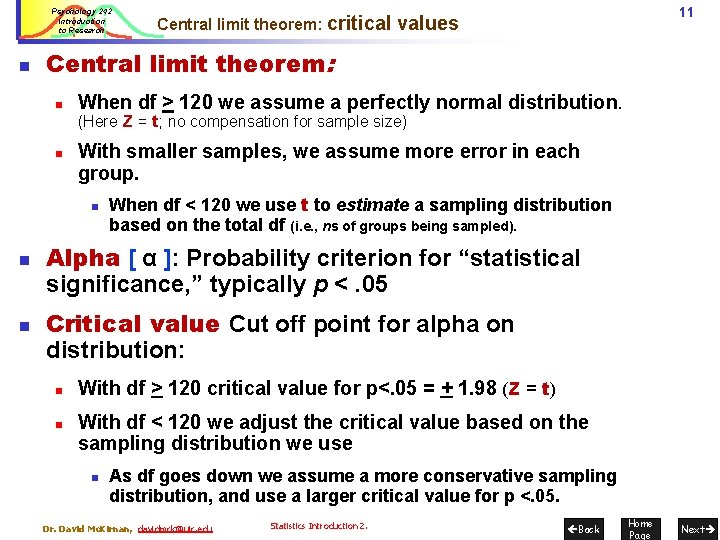
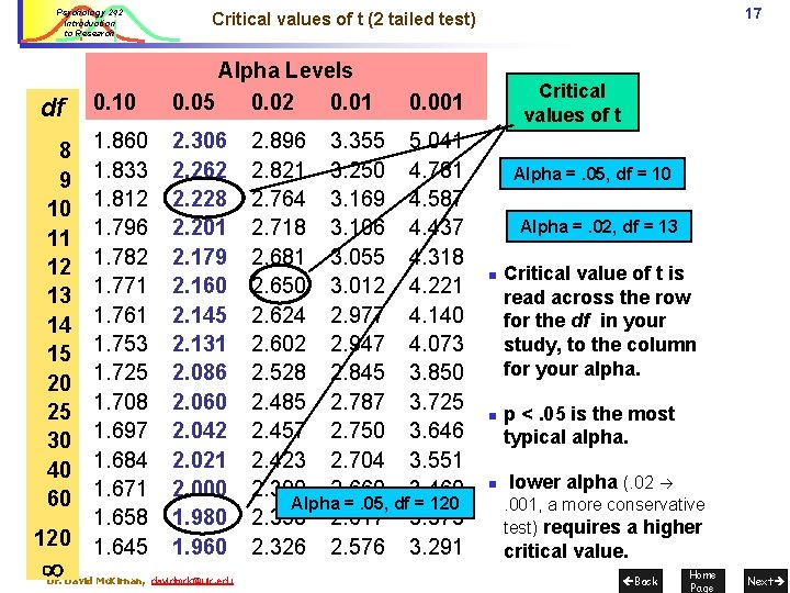
Psychology 242 Introduction to Research n n When df > 120 we assume a perfectly normal distribution. (Here Z = t; no compensation for sample size) With smaller samples, we assume more error in each group. n n 11 values Central limit theorem: n n Central limit theorem: critical When df < 120 we use t to estimate a sampling distribution based on the total df (i. e. , ns of groups being sampled). Alpha [ α ]: Probability criterion for “statistical significance, ” typically p <. 05 Critical value Cut off point for alpha on distribution: n n With df > 120 critical value for p<. 05 = + 1. 98 (Z = t) With df < 120 we adjust the critical value based on the sampling distribution we use n As df goes down we assume a more conservative sampling distribution, and use a larger critical value for p <. 05. Dr. David Mc. Kirnan, davidmck@uic. edu Statistics Introduction 2. Back Home Page Next

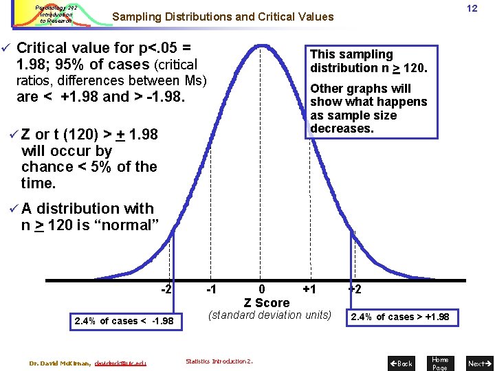
Psychology 242 Introduction to Research 12 Sampling Distributions and Critical Values ü Critical value for p<. 05 = 1. 98; 95% of cases (critical ratios, differences between Ms) This sampling distribution n > 120. Other graphs will show what happens as sample size decreases. are < +1. 98 and > -1. 98. ü Z or t (120) > + 1. 98 will occur by chance < 5% of the time. ü A distribution with n > 120 is “normal” -2 2. 4% of cases < -1. 98 Dr. David Mc. Kirnan, davidmck@uic. edu -1 0 Z Score +1 (standard deviation units) Statistics Introduction 2. +2 2. 4% of cases > +1. 98 Back Home Page Next

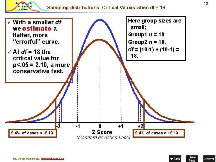
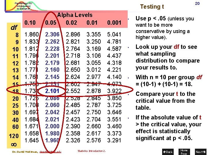
Psychology 242 Introduction to Research 13 Sampling distributions: Critical Values when df = 18 Here group sizes are small; Group 1 n = 10 Group 2 n = 10. df = (10 -1) + (10 -1) = 18. ü With a smaller df we estimate a flatter, more “errorful” curve. ü At df = 18 the critical value for p<. 05 = 2. 10, a more conservative test. -2 2. 4% of cases < -2. 10 Dr. David Mc. Kirnan, davidmck@uic. edu -1 0 Z Score +1 (standard deviation units) +2 2. 4% of cases > +2. 10 Back Home Page Next

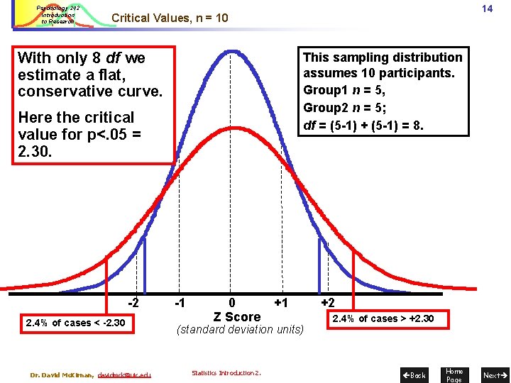
Psychology 242 Introduction to Research 14 Critical Values, n = 10 With only 8 df we estimate a flat, conservative curve. This sampling distribution assumes 10 participants. Group 1 n = 5, Group 2 n = 5; df = (5 -1) + (5 -1) = 8. Here the critical value for p<. 05 = 2. 30. -2 2. 4% of cases < -2. 30 Dr. David Mc. Kirnan, davidmck@uic. edu -1 0 Z Score +1 (standard deviation units) Statistics Introduction 2. +2 2. 4% of cases > +2. 30 Back Home Page Next

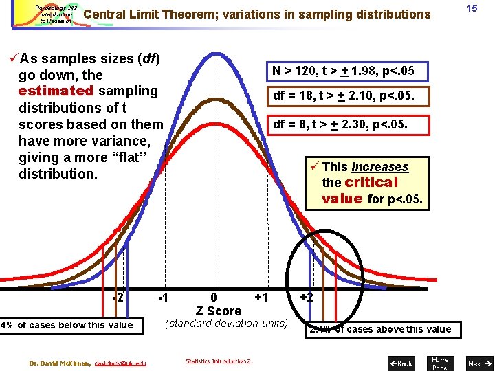
Psychology 242 Introduction to Research 15 Central Limit Theorem; variations in sampling distributions üAs samples sizes (df) go down, the estimated sampling distributions of t scores based on them have more variance, giving a more “flat” distribution. -2 . 4% of cases below this value Dr. David Mc. Kirnan, davidmck@uic. edu N > 120, t > + 1. 98, p<. 05 df = 18, t > + 2. 10, p<. 05. df = 8, t > + 2. 30, p<. 05. ü This increases the critical value for p<. 05. -1 0 Z Score +1 (standard deviation units) Statistics Introduction 2. +2 2. 4% of cases above this value Back Home Page Next

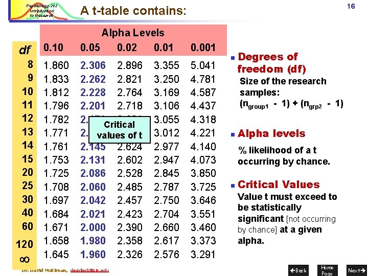
Psychology 242 Introduction to Research df 0. 10 8 9 10 11 12 13 14 15 20 25 30 40 60 1. 833 1. 812 1. 796 1. 782 1. 771 1. 761 1. 753 1. 725 1. 708 1. 697 1. 684 1. 671 1. 658 1. 645 120 16 A t-table contains: Alpha Levels 0. 05 0. 02 0. 01 2. 306 2. 896 2. 262 2. 821 2. 228 2. 764 2. 201 2. 718 2. 179 Critical 2. 681 2. 160 2. 650 values of t 2. 145 2. 624 2. 131 2. 602 2. 086 2. 528 2. 060 2. 485 2. 042 2. 457 2. 021 2. 423 2. 000 2. 390 1. 980 2. 358 1. 960 2. 326 Dr. David Mc. Kirnan, davidmck@uic. edu 3. 355 3. 250 3. 169 3. 106 3. 055 3. 012 2. 977 2. 947 2. 845 2. 787 2. 750 2. 704 2. 660 2. 617 2. 576 0. 001 5. 041 4. 781 4. 587 4. 437 4. 318 4. 221 4. 140 4. 073 3. 850 3. 725 3. 646 3. 551 3. 460 3. 373 3. 291 n Degrees of freedom (df) Size of the research samples: (ngroup 1 - 1) + (ngrp 2 - 1) n Alpha levels % likelihood of a t occurring by chance. n Critical Values Value t must exceed to be statistically significant [not occurring by chance] at a given alpha. Back Home Page Next

Psychology 242 Introduction to Research df 0. 10 Alpha Levels 0. 05 0. 02 0. 01 8 9 10 11 12 13 14 15 20 25 30 40 60 1. 833 1. 812 1. 796 1. 782 1. 771 1. 761 1. 753 1. 725 1. 708 1. 697 1. 684 1. 671 1. 658 1. 645 2. 306 2. 262 2. 228 2. 201 2. 179 2. 160 2. 145 2. 131 2. 086 2. 060 2. 042 2. 021 2. 000 1. 980 1. 960 120 17 Critical values of t (2 tailed test) Dr. David Mc. Kirnan, davidmck@uic. edu Critical values of t 0. 001 2. 896 3. 355 5. 041 2. 821 3. 250 4. 781 2. 764 3. 169 4. 587 2. 718 3. 106 4. 437 2. 681 3. 055 4. 318 2. 650 3. 012 4. 221 2. 624 2. 977 4. 140 2. 602 2. 947 4. 073 2. 528 2. 845 3. 850 2. 485 2. 787 3. 725 2. 457 2. 750 3. 646 2. 423 2. 704 3. 551 2. 390 2. 660 3. 460 Alpha =. 05, df = 120 2. 358 2. 617 3. 373 2. 326 2. 576 3. 291 Alpha =. 05, df = 10 Alpha =. 02, df = 13 n n n Critical value of t is read across the row for the df in your study, to the column for your alpha. p <. 05 is the most typical alpha. lower alpha (. 02 . 001, a more conservative test) requires a higher critical value. Back Home Page Next

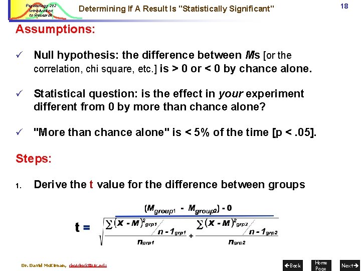
Psychology 242 Introduction to Research 18 Determining If A Result Is "Statistically Significant" Assumptions: ü Null hypothesis: the difference between Ms [or the correlation, chi square, etc. ] is > 0 or < 0 by chance alone. ü Statistical question: is the effect in your experiment different from 0 by more than chance alone? ü "More than chance alone" is < 5% of the time [p <. 05]. Steps: 1. Derive the t value for the difference between groups Dr. David Mc. Kirnan, davidmck@uic. edu Back Home Page Next

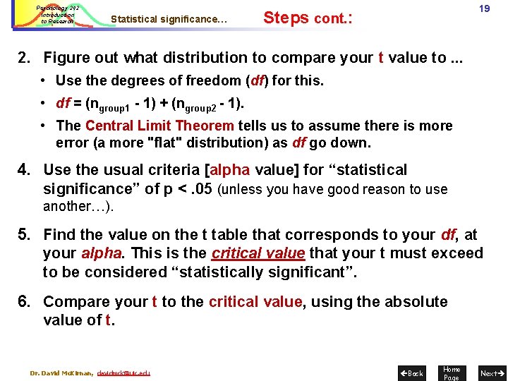
Psychology 242 Introduction to Research Statistical significance… 19 Steps cont. : 2. Figure out what distribution to compare your t value to. . . • Use the degrees of freedom (df) for this. • df = (ngroup 1 - 1) + (ngroup 2 - 1). • The Central Limit Theorem tells us to assume there is more error (a more "flat" distribution) as df go down. 4. Use the usual criteria [alpha value] for “statistical significance” of p <. 05 (unless you have good reason to use another…). 5. Find the value on the t table that corresponds to your df, at your alpha. This is the critical value that your t must exceed to be considered “statistically significant”. 6. Compare your t to the critical value, using the absolute value of t. Dr. David Mc. Kirnan, davidmck@uic. edu Back Home Page Next

Psychology 242 Introduction to Research df 8 9 10 11 12 13 14 15 18 20 25 30 40 60 120 20 Testing t 0. 10 Alpha Levels 0. 05 0. 02 0. 01 0. 001 1. 860 1. 833 1. 812 1. 796 1. 782 1. 771 1. 761 1. 753 1. 734 1. 725 1. 708 1. 697 1. 684 1. 671 1. 658 1. 645 2. 306 2. 262 2. 228 2. 201 2. 179 2. 160 2. 145 2. 131 2. 101 2. 086 2. 060 2. 042 2. 021 2. 000 1. 980 1. 960 5. 041 4. 781 4. 587 4. 437 4. 318 4. 221 4. 140 4. 073 3. 922 3. 850 3. 725 3. 646 3. 551 3. 460 3. 373 3. 291 Dr. David Mc. Kirnan, davidmck@uic. edu 2. 896 2. 821 2. 764 2. 718 2. 681 2. 650 2. 624 2. 602 2. 552 2. 528 2. 485 2. 457 2. 423 2. 390 2. 358 2. 326 3. 355 3. 250 3. 169 3. 106 3. 055 3. 012 2. 977 2. 947 2. 878 2. 845 2. 787 2. 750 2. 704 2. 660 2. 617 2. 576 Statistics Introduction 2. • Use p <. 05 (unless you want to be more conservative by using a higher value). • • Look up your df to see what sampling distribution to compare your results to. With n = 10 per group df = (10 -1) + (10 -1) = 18. Compare your t to the critical value from the table. If the absolute value of t > the critical value, your effect is statistically significant at p <. 05. Back Home Page Next