Parallel computations based on numerical Nadpis 1 integration

Parallel computations based on numerical Nadpis 1 integration methods Nadpis 2 Nadpis 3 Jméno Jiří Kunovský Příjmení Vysoké učení technické v Brně, Fakulta informačních technologií v Brně Vysoké učení technické v Brně, Fakulta informačních technologií Božetěchova 2, 612 66 Brno jmeno@fit. vutbr. cz kunovsky@fit. vutbr. cz 99. 2008

Abstract Extremely Accurate Solutions of Systems of Differential Equations The development project deals with extremely exact, stable and fast numerical solutions of systems of differential equations. www. itsolution. cz/TKSL 2

Abstract The project is based on a mathematical method which uses the Taylor series method for solving differential equations. www. itsolution. cz/TKSL 3

Introduction The best-known and most accurate method of calculating a new value of a numerical solution of a differential equation is to construct the Taylor series in the form www. itsolution. cz/TKSL 4

Taylor Series Method www. itsolution. cz/TKSL 5

Modern Taylor Series Method An important part of the method is an automatic integration order setting, i. e. using as many Taylor series terms as the defined accuracy requires. www. itsolution. cz/TKSL 6

Fourier a 1'=k*f*cos(t) & 0; a 3'=k*f*cos(3*t) & 0; www. itsolution. cz/TKSL 7

There are many approaches how to compute numerical integrations in parallel in MATLAB and MAPLE

Fourier 1 var y, z, u, v, x, f, f 1, f 2, a 0, a 1, a 2, a 3, a 4, a 5, a 6, b 0, b 1, b 2, b 3, b 4, b 5, vysl, ys 1, ys 2, ys 3, ys 5, yc 1, yc 3, v 1, v 2, v 3, v 4, v 5; Const PI=3. 1415926535897932385, om=1, eps=1 e 20, tmax=2*PI, k=1/PI; system f=0. 33*cos(t)+ 2*cos(2*t)+0. 8 *sin(t)+ 2. 5*sin(2*t); b 1'=k*f*sin(om*t) &0; a 1'=k*f*cos(om*t) &0; b 2'=k*f*sin(2*om*t) &0; a 2'=k*f*cos(2*om*t) &0; a 3'=k*f*cos(3*om*t) &0; b 3'=k*f*sin(3*om*t) &0; a 4'=k*f*cos(4*om*t) &0; b 4'=k*f*sin(4*om*t) &0; a 5'=k*f*cos(5*om*t) &0; b 5'=k*f*sin(5*om*t) &0; a 6'=k*f*cos(6*om*t) &0; sysend. www. itsolution. cz/TKSL 9

Fourier 1 www. itsolution. cz/TKSL 10

Fourier 1 f=0. 33*cos(t)+ 2*cos(2*t)+0. 8 *sin(t)+ 2. 5*sin(2*t); www. itsolution. cz/TKSL 11

Fourier 1 f=0. 33*cos(t)+ 2*cos(2*t)+0. 8 *sin(t)+ 2. 5*sin(2*t); www. itsolution. cz/TKSL 12

Fourier 1 f=0. 33*cos(t)+ 2*cos(2*t)+0. 8 *sin(t)+ 2. 5*sin(2*t); www. itsolution. cz/TKSL 13

Fourier 2 var f, a 0, a 1, a 2, a 3, a 4, a 5, b 0, b 1, b 2, b 3, b 4, b 5; const PI=3. 1415926535897932385, om=1, eps=1 e-20, tmax=2*PI, k=1/PI; system f=16*sin(t)*sin(t)*sin(t)+4*cos(t)*cos(t) -sin(t)*sin(t)+cos(t)*cos(t)+2*sin(t)*cos(t)-sin(5*t) +5*sin(3*t) -cos(3*t)-cos(2*t)-sin(2*t)-10*sin(t); b 1'=k*f*sin(om*t) &0; a 1'=k*f*cos(om*t) &0; b 2'=k*f*sin(2*om*t) &0; a 2'=k*f*cos(2*om*t) &0; a 3'=k*f*cos(3*om*t) &0; b 3'=k*f*sin(3*om*t) &0; a 4'=k*f*cos(4*om*t) &0; b 4'=k*f*sin(4*om*t) &0; a 5'=k*f*cos(5*om*t) &0; b 5'=k*f*sin(5*om*t) &0; sysend. f=3*cos(t); ? ? www. itsolution. cz/TKSL 14

Fourier 2 f=3*cos(t); www. itsolution. cz/TKSL 15

Fourier 2 f=3*cos(t); www. itsolution. cz/TKSL 16

Fourier 2 f=3*cos(t); www. itsolution. cz/TKSL 17

Finite Integrals – Example 1 f'=sin(t) www. itsolution. cz/TKSL 18

Finite Integrals – Example 1 var f; const dt=0. 1, tmax=pi, eps=1 e-20; system f'=sin(t) &0; sysend. www. itsolution. cz/TKSL 19

Finite Integrals – Example 1 www. itsolution. cz/TKSL 20

Finite Integrals – Example 2 f'=t*t/(t*t+1) www. itsolution. cz/TKSL 21

Finite Integrals – Example 2 var f; const dt=0. 1, tmax=1, eps=1 e-20; system f'=t*t/(t*t+1) &0; sysend. www. itsolution. cz/TKSL 22

Finite Integrals – Example 2 www. itsolution. cz/TKSL 23

Finite Integrals – Example 3 f'=sin(t)*cos(t) www. itsolution. cz/TKSL 24

Finite Integrals – Example 3 var f; const dt=0. 1, tmax=pi/2, eps=1 e-20; system f'=sin(t)*cos(t) &0; sysend. www. itsolution. cz/TKSL 25

Finite Integrals – Example 3 www. itsolution. cz/TKSL 26

Finite Integrals – Example 4 f'=3*sin(t)*cos(t) www. itsolution. cz/TKSL 27

Finite Integrals – Example 4 var f; const dt=0. 1, tmax=pi/2, eps=1 e-20; system f'=3*sin(t)*cos(t) &0; sysend. www. itsolution. cz/TKSL 28

Finite Integrals – Example 4 www. itsolution. cz/TKSL 29

Finite Integrals – Example 5 f'=t*sin(t) www. itsolution. cz/TKSL 30

Finite Integrals – Example 5 var f; const dt=0. 1, tmax=2*pi, eps=1 e-20; system f'=t*sin(t) &0; sysend. www. itsolution. cz/TKSL 31

Finite Integrals – Example 5 www. itsolution. cz/TKSL 32

Finite Integrals – Example 6 f'=1/pi*t*sin(t) www. itsolution. cz/TKSL 33

Finite Integrals – Example 6 var f; const dt=0. 1, tmax=2*pi, eps=1 e-20; system f'=1/pi*t*sin(t) &0; sysend. www. itsolution. cz/TKSL 34

Finite Integrals – Example 6 www. itsolution. cz/TKSL 35

A special transformation into elementary representation is expected www. itsolution. cz/TKSL 36

Everything is based on numerical inntegration methods, of course It is very important to rewrite the original form y' = f(t, y) into a special form – for every equtation www. itsolution. cz/TKSL 37

The first order homogenous differential equtations is presented as an example y' – y = 0 y(0) = y 0 or y' = y Euler method gives new value y i + 1 = yi + h*y'i which is equal to y i + 1 = yi + h*yi

Computation starts from initial condition y(0) = y 0 it means y = y + h*y 1 0 0 Similarly y 2 = y 1 + h*y 1 y 3 = y 2 + h*y 2 . . .

Correspending circuit representation y 1 = y 0 + h * y 0 output y 0 CLK ADD y 0 * y 0 h www. itsolution. cz/TKSL 40

Well-known analog integrator y(0) CLK y 0 output ADD * y 0 h www. itsolution. cz/TKSL 41

Parallel data bus in Euler integrator

Automatic transformation An automatic transformation of the original problem is a necessary part of the Modern Taylor Series Method. The original system of differential equations is automatically transformed to a polynomial form, i. e. to a form suitable for easily calculating the Taylor series forms using recurrent formulae. www. itsolution. cz/TKSL 46

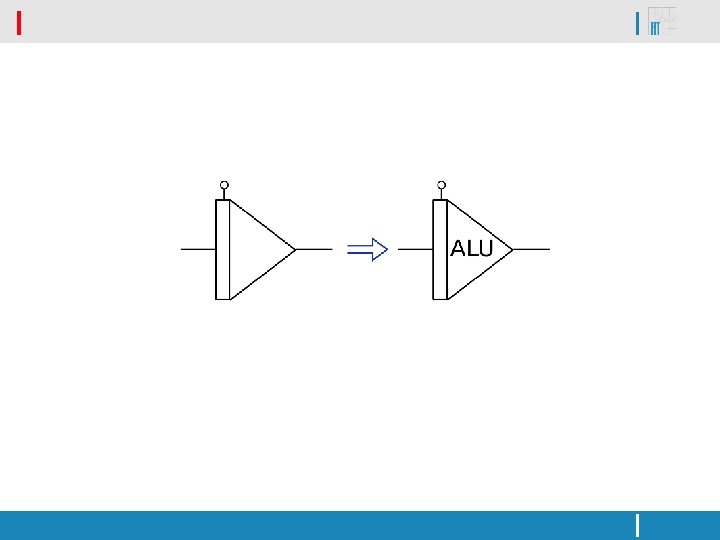
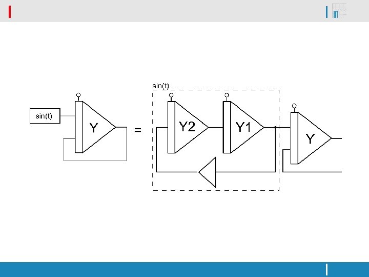
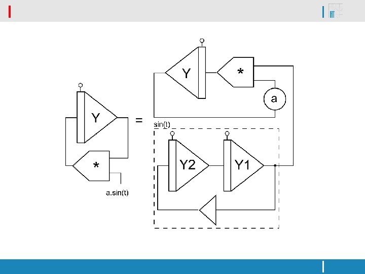
Transformation of differential equation www. itsolution. cz/TKSL 47

Transformation of differential equation www. itsolution. cz/TKSL 48

Transformation of differential equation www. itsolution. cz/TKSL 49

Transformation of differential equation www. itsolution. cz/TKSL 50

Results www. itsolution. cz/TKSL 51

Results www. itsolution. cz/TKSL 52

Results www. itsolution. cz/TKSL 53

Results 6 integrators (processors) www. itsolution. cz/TKSL 54

Integration step - asymptote h=0. 1 h=0. 001 www. itsolution. cz/TKSL 55

An Exponential Test Example • Analytic solution www. itsolution. cz/TKSL 56

Experiments The TKSL is used for the experiments. For a given integration step dt, the method order ORD is automatically determined during computation. • Theoretically, the calculation can be done with an arbitrary integration step. • The resulting solutions are of course identical only the order ORD used by the method changes. For a small integration step dt, the method order ORD may be small, and, as the integration step increases, obviously, the method order must be higher. www. itsolution. cz/TKSL 57

An Exponential Test Example (h=0. 01) www. itsolution. cz/TKSL 58

An Exponential Test Example (h=0. 1) www. itsolution. cz/TKSL 59

An Exponential Test Example (h=1) www. itsolution. cz/TKSL 60

An Exponential Test Example, A=0. 1 A = 0. 1 TKSL ORDER = 4 www. itsolution. cz/TKSL 61

An Exponential Test Example, A=1 TKSL ORDER = 4 www. itsolution. cz/TKSL 62

An Exponential Test Example, A=10 TKSL ORDER = 4 www. itsolution. cz/TKSL 63

Van der Pol’s Equation www. itsolution. cz/TKSL 64

Van der Pol’s Equation www. itsolution. cz/TKSL 65

Experiments Thus it is usual that the computation uses different numbers of Taylor series terms for different steps of constant length. www. itsolution. cz/TKSL 66

Van der Pol’s Equation www. itsolution. cz/TKSL 67

Van der Pol’s Equation www. itsolution. cz/TKSL 68

Van der Pol’s Equation www. itsolution. cz/TKSL 69

Van der Pol’s Equation www. itsolution. cz/TKSL 70

Stiff systems - definition • Problems where explicit methods doesn`t work. [Hairer, Wanner 1996] • Stiffness ratio: … eigenvalues of Jacobian www. itsolution. cz/TKSL 71

Stiff systems - example www. itsolution. cz/TKSL 72

Stiff systems - example a=1 www. itsolution. cz/TKSL 73

Stiff systems - example a = 5000 www. itsolution. cz/TKSL 74

Stiff exponential y’ = z z’ = -ay –(a+1)z &1 &-1 Analytic solution Stiffness ratio y = e-t z = -e-t r=a www. itsolution. cz/TKSL 75

Stiff exponential (a=100) y’ = z z’ = -100 y -101 z &1 &-1 h=1 DY 1 = h z DZ 1 = h(-100 y -101 z) DY 1 = -1 DZ 1 = -100+101 = 1 www. itsolution. cz/TKSL 76

Stiff exponential (a=100) y’ = z z’ = -100 y -101 z DY 2 = h/2 DZ 1 DY 2 = 0. 5 &1 &-1 h=1 DZ 2 = h/2(-100 DY 1 -101 DZ 1) DZ 2 = 0. 5(100 -101) = -0. 5 www. itsolution. cz/TKSL 77

Stiff exponential (a=100) y’ = z z’ = -100 y -101 z DY 3 = h/3 DZ 2 DY 3 = -0. 5/3 &1 &-1 h=1 DZ 3 = h/3(-100 DY 2 -101 DZ 2) DZ 3 = 1/3(-50+101∙ 0. 5) DY 3 = -0. 16666 DZ 3 = 0. 16666 www. itsolution. cz/TKSL 78

Stiff exponential (a=100) y’ = z z’ = -100 y -101 z DY 4 = h/4 DZ 3 DY 4 = 1/4 (0. 16666) DY 4 = 0. 041666666 &1 &-1 h=1 DZ 4 = h/4(-100 DY 3 -101 DZ 3) DZ 4 = 1/4(16. 6666666 – 16. 83333327) DZ 4 = -0. 041666666 www. itsolution. cz/TKSL 79

Stiff exponential (a=106) y’ = z &1 z’ = -1000000 y -1000001 z DY 1 = h z DY 1 = -1 &-1 h=1 DZ 1 = h(-1000000 y 1000001 z) DZ 1 = 1 www. itsolution. cz/TKSL 80

Stiff exponential (a=106) y’ = z &1 z’ = -1000000 y -1000001 z DY 2 = h/2 DZ 1 DY 2 = 0. 5 &-1 h=1 DZ 2 = h/2(-1000000 DY 11000001 DZ 1) DZ 2 = -0. 5 www. itsolution. cz/TKSL 81

Stiff exponential (a=106) y’ = z &1 z’ = -1000000 y -1000001 z DY 3 = h/3 DZ 2 DY 3 = 0. 16666 &-1 h=1 DZ 3 = h/3(-1000000 DY 21000001 DZ 2) DZ 3 = 0. 16666 www. itsolution. cz/TKSL 82

Stiff exponential (a=106) y’ = z &1 z’ = -1000000 y -1000001 z &-1 h=1 DY 4 = h/4 DZ 3 DZ 4 = h/4(-1000000 DY 31000001 DZ 3) DY 4 = 0. 041666666 DZ 4 =1/4(166666. 666166666. 8327) DZ 4 = -0. 041675 www. itsolution. cz/TKSL 83

Stiff exponential (a=106) y’ = z &1 z’ = -1000000 y -1000001 z DY 5 = h/5 DZ 4 DY 5 = -0. 008335 |DY 5|=|DZ 5| &-1 h=1 DZ 5 = h/5(-1000000 DY 41000001 DZ 4) DZ 5 =1/5(-41666. 666+ 41675. 04168) DZ 5 = 1. 675115 www. itsolution. cz/TKSL 84

Stiff exponential (a=106) y’ = z &1 z’ = -1000000 y -1000001 z &-1 h=1 DY 6 = h/6 DZ 5 DZ 6 = h/6(-1000000 DY 51000001 DZ 5) DY 6 = 0. 279189166 DZ 6 =1/6(-8335167513. 675) DZ 5 = -280578. 6125 www. itsolution. cz/TKSL 85

Stiff exponential – multiple arithmetic a bits 1010 3681 1020 8900 1050 24000 www. itsolution. cz/TKSL 86

Problem 2 y'=L*(y-sin(t))+cos(t) &0; Analytic solution y = sin(t) www. itsolution. cz/TKSL 87

Problem 2 (L=108) ORD hmax 6 0. 00625 8 0. 0125 10 0. 05 12 0. 125 14 0. 25 18 0. 5 64 10 www. itsolution. cz/TKSL 88

Conclusion Extremely Accurate Solutions of Systems of Differential Equations The development project deals with extremely exact, stable and fast numerical solutions of systems of differential equations. www. itsolution. cz/TKSL 89

Thank you for attention! www. itsolution. cz/TKSL 90