15 EXCHANGE RATES II THE ASSET APPROACH IN

15 EXCHANGE RATES II: THE ASSET APPROACH IN THE SHORT RUN 1 Exchange Rates and Interest Rates in the Short Run 2 Interest Rates in the Short Run 3 The Asset Approach 4 A Complete Theory 5 Fixed Exchange Rates and the Trilemma 6 Conclusions

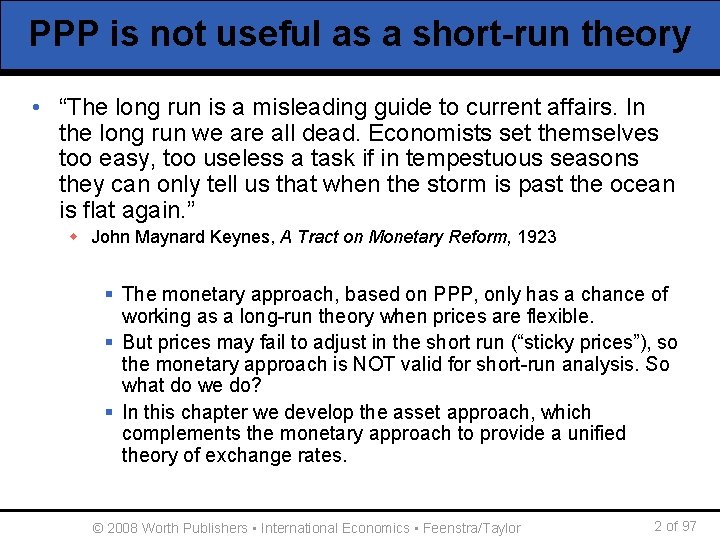
PPP is not useful as a short-run theory • “The long run is a misleading guide to current affairs. In the long run we are all dead. Economists set themselves too easy, too useless a task if in tempestuous seasons they can only tell us that when the storm is past the ocean is flat again. ” w John Maynard Keynes, A Tract on Monetary Reform, 1923 § The monetary approach, based on PPP, only has a chance of working as a long-run theory when prices are flexible. § But prices may fail to adjust in the short run (“sticky prices”), so the monetary approach is NOT valid for short-run analysis. So what do we do? § In this chapter we develop the asset approach, which complements the monetary approach to provide a unified theory of exchange rates. © 2008 Worth Publishers ▪ International Economics ▪ Feenstra/Taylor 2 of 97

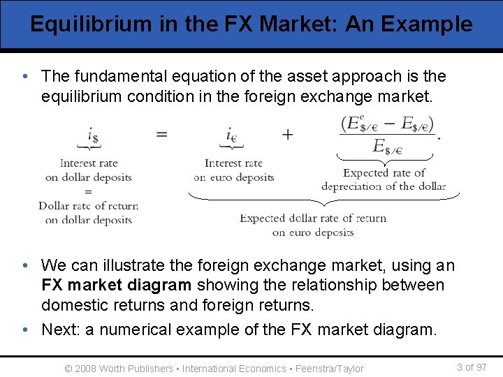
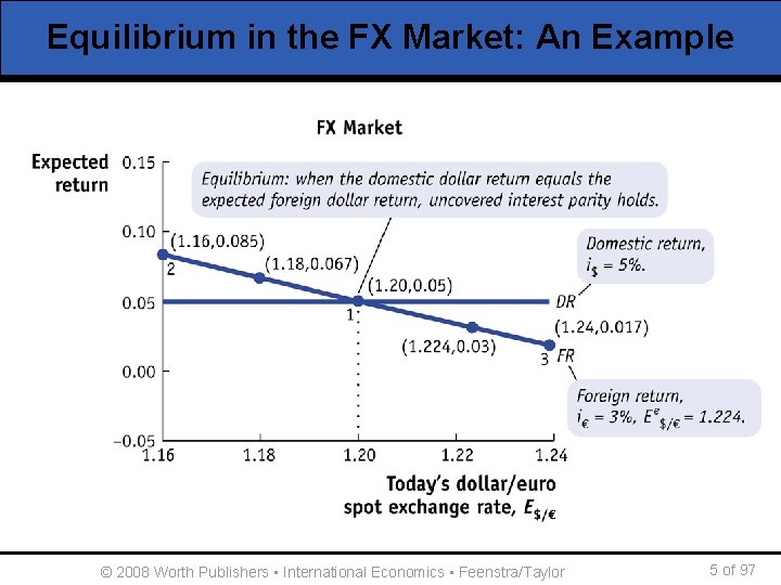
Equilibrium in the FX Market: An Example • The fundamental equation of the asset approach is the equilibrium condition in the foreign exchange market. • We can illustrate the foreign exchange market, using an FX market diagram showing the relationship between domestic returns and foreign returns. • Next: a numerical example of the FX market diagram. © 2008 Worth Publishers ▪ International Economics ▪ Feenstra/Taylor 3 of 97

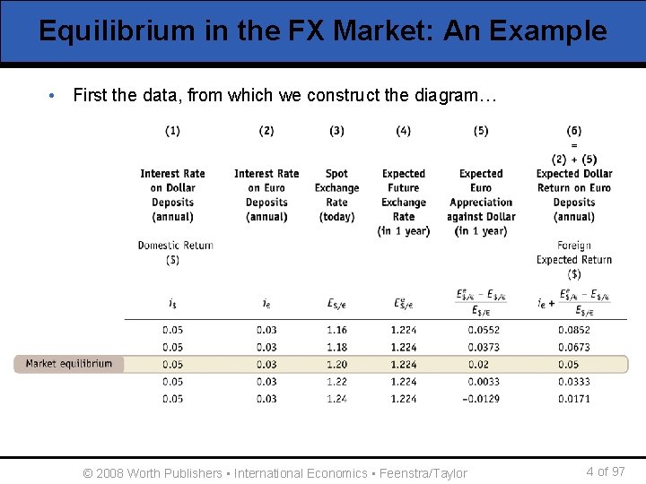
Equilibrium in the FX Market: An Example • First the data, from which we construct the diagram… © 2008 Worth Publishers ▪ International Economics ▪ Feenstra/Taylor 4 of 97

Equilibrium in the FX Market: An Example © 2008 Worth Publishers ▪ International Economics ▪ Feenstra/Taylor 5 of 97

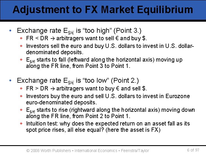
Adjustment to FX Market Equilibrium • Exchange rate E$/€ is “too high” (Point 3. ) w FR < DR → arbitragers want to sell € and buy $. w Investors sell the euro and buy U. S. dollars to invest in U. S. dollardenominated deposits. w E$/€ starts to fall (leftward along the horizontal axis) moving up along the FR line, from Point 3 to Point 1. • Exchange rate E$/€ is “too low” (Point 2. ) w FR > DR → arbitragers want to buy € and sell $. w Investors buy the euro and sell U. S. dollars to invest in Eurozone euro-denominated deposits. w E$/€ starts to rise (rightward along the horizontal axis) moving down along the FR line, from Point 2 to Point 1. w Intuition test: why does the expected return on an asset fall as its spot price rises, all else equal? (here the asset is FX) © 2008 Worth Publishers ▪ International Economics ▪ Feenstra/Taylor 6 of 97

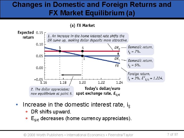
Changes in Domestic and Foreign Returns and FX Market Equilibrium (a) • Increase in the domestic interest rate, i$ w DR shifts upward. w E$/€ decreases (home currency appreciates). © 2008 Worth Publishers ▪ International Economics ▪ Feenstra/Taylor 7 of 97

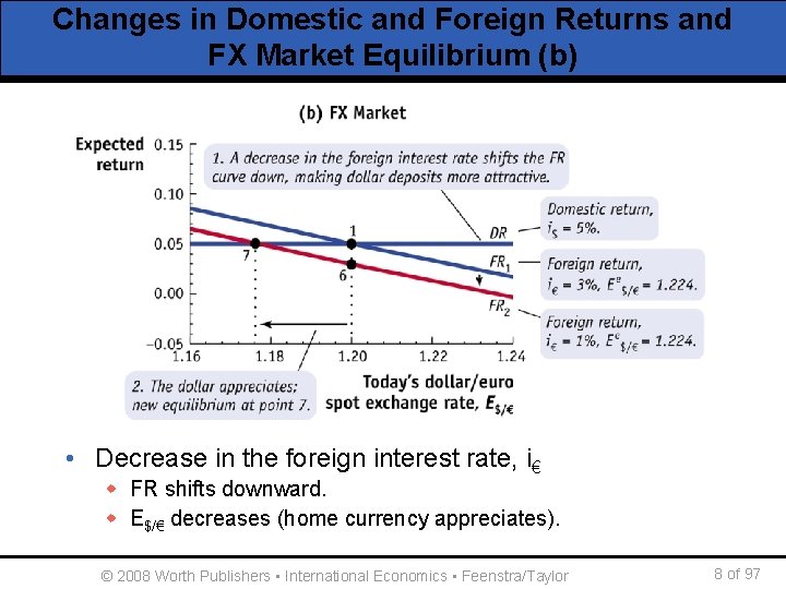
Changes in Domestic and Foreign Returns and FX Market Equilibrium (b) • Decrease in the foreign interest rate, i€ w FR shifts downward. w E$/€ decreases (home currency appreciates). © 2008 Worth Publishers ▪ International Economics ▪ Feenstra/Taylor 8 of 97

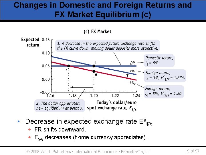
Changes in Domestic and Foreign Returns and FX Market Equilibrium (c) • Decrease in expected exchange rate Ee$/€ w FR shifts downward. w E$/€ decreases (home currency appreciates). © 2008 Worth Publishers ▪ International Economics ▪ Feenstra/Taylor 9 of 97

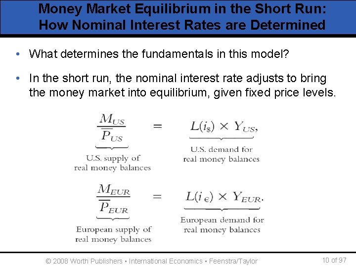
Money Market Equilibrium in the Short Run: How Nominal Interest Rates are Determined • What determines the fundamentals in this model? • In the short run, the nominal interest rate adjusts to bring the money market into equilibrium, given fixed price levels. © 2008 Worth Publishers ▪ International Economics ▪ Feenstra/Taylor 10 of 97

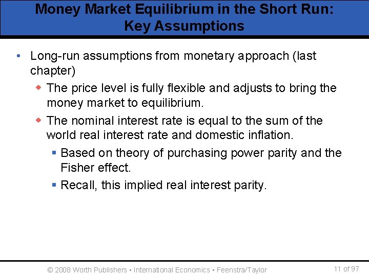
Money Market Equilibrium in the Short Run: Key Assumptions • Long-run assumptions from monetary approach (last chapter) w The price level is fully flexible and adjusts to bring the money market to equilibrium. w The nominal interest rate is equal to the sum of the world real interest rate and domestic inflation. § Based on theory of purchasing power parity and the Fisher effect. § Recall, this implied real interest parity. © 2008 Worth Publishers ▪ International Economics ▪ Feenstra/Taylor 11 of 97

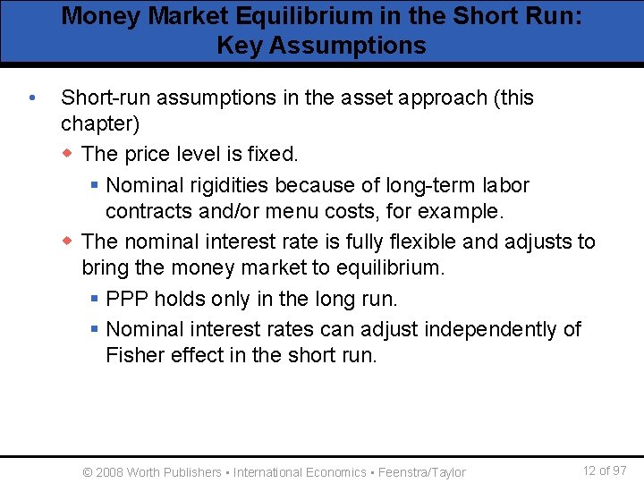
Money Market Equilibrium in the Short Run: Key Assumptions • Short-run assumptions in the asset approach (this chapter) w The price level is fixed. § Nominal rigidities because of long-term labor contracts and/or menu costs, for example. w The nominal interest rate is fully flexible and adjusts to bring the money market to equilibrium. § PPP holds only in the long run. § Nominal interest rates can adjust independently of Fisher effect in the short run. © 2008 Worth Publishers ▪ International Economics ▪ Feenstra/Taylor 12 of 97

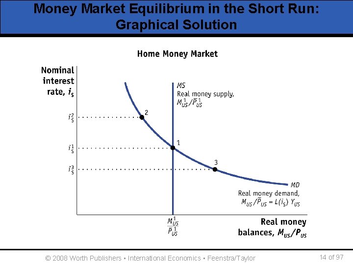
Money Market Equilibrium in the Short Run: Graphical Solution • Supply of real money balances. w M is set by the central bank. w P is assumed to be fixed in the short run. w Notice, both of these variables are independent of the nominal interest rate. Therefore, the money supply (MS) curve is vertical. • Demand for real money balances. w Money demand is a decreasing function of the nominal interest rate opportunity cost. w Since the quantity of real money balances demanded decreases with an increase in the nominal interest rate, the money demand curve is downward sloping. © 2008 Worth Publishers ▪ International Economics ▪ Feenstra/Taylor 13 of 97

Money Market Equilibrium in the Short Run: Graphical Solution © 2008 Worth Publishers ▪ International Economics ▪ Feenstra/Taylor 14 of 97

Adjustment to Money Market Equilibrium in the Short Run • Suppose interest rates are “too high” (point 2): w Excess money supply. § The public will want to reduce cash holdings by exchanging money for assets such as bonds, saving accounts etc. That is, they will save more and seek to lend their money to borrowers. § But borrowers will not want borrow more unless the cost of borrowing falls. • When the interest rate is “too low” (point 3): w Excess money demand. § The public will want to increase cash holdings by exchanging interest-bearing assets for money. That is, they will save less and reduce the amount available to borrowers. § But borrowers want to borrow the same amount. © 2008 Worth Publishers ▪ International Economics ▪ Feenstra/Taylor 15 of 97

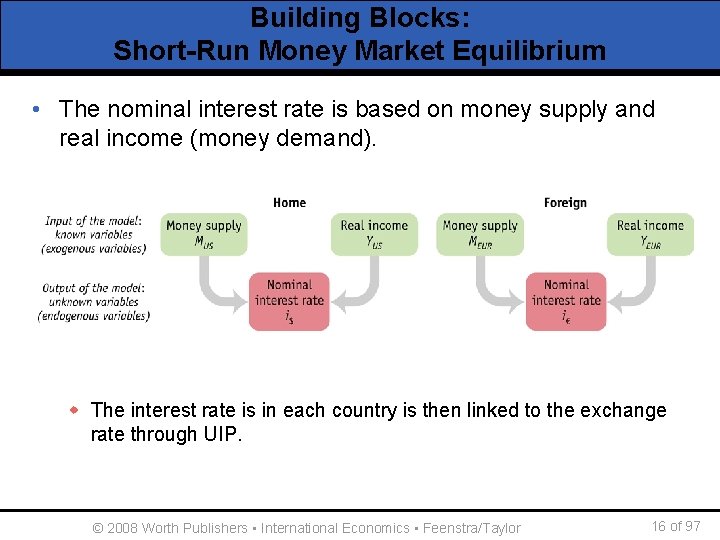
Building Blocks: Short-Run Money Market Equilibrium • The nominal interest rate is based on money supply and real income (money demand). w The interest rate is in each country is then linked to the exchange rate through UIP. © 2008 Worth Publishers ▪ International Economics ▪ Feenstra/Taylor 16 of 97

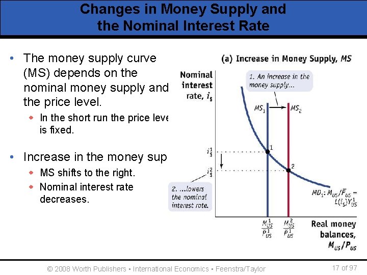
Changes in Money Supply and the Nominal Interest Rate • The money supply curve (MS) depends on the nominal money supply and the price level. w In the short run the price level is fixed. • Increase in the money supply. w MS shifts to the right. w Nominal interest rate decreases. © 2008 Worth Publishers ▪ International Economics ▪ Feenstra/Taylor 17 of 97

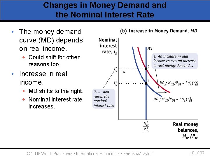
Changes in Money Demand the Nominal Interest Rate • The money demand curve (MD) depends on real income. w Could shift for other reasons too. • Increase in real income. w MD shifts to the right. w Nominal interest rate increases. © 2008 Worth Publishers ▪ International Economics ▪ Feenstra/Taylor 18 of 97

Money Market Equilibrium: The Short Run versus the Long Run • Note: short-run analysis gives results that differ significantly from those we found using the monetary approach in the long run. w This chapter versus last chapter. • Thus, in applications, it is important to distinguish between temporary shocks and permanent shocks. w Temporary shocks dissipate before prices adjust. Therefore, they affect the economy only in the short run. § Expectations for the future will remain unaffected. w Permanent shocks affect the economy in the long run, so that price adjustment will occur. § And expectations will be affected. © 2008 Worth Publishers ▪ International Economics ▪ Feenstra/Taylor 19 of 97

Money Market Equilibrium: The Short Run versus the Long Run • Example: A central bank that had previously kept the money supply constant, now lets M grow at 5% per year. w In the long run, the predictions of the long-run monetary model and Fisher effect are clear. § All else equal, a 5 percentage point increase in the rate of money growth causes a 5 percentage point increase in the rate of inflation, and § a 5 percentage point increase in the nominal interest rate. The home interest rate will rise in the long run. w In the short run, the model tells a very different story. § If the money supply expands, the immediate effect is an excess supply of real money balances. § The home interest rate will fall in the short run. © 2008 Worth Publishers ▪ International Economics ▪ Feenstra/Taylor 20 of 97

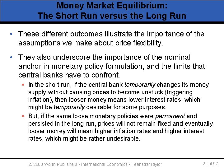
Money Market Equilibrium: The Short Run versus the Long Run • These different outcomes illustrate the importance of the assumptions we make about price flexibility. • They also underscore the importance of the nominal anchor in monetary policy formulation, and the limits that central banks have to confront. w In the short run, if the central bank temporarily changes its money supply without causing prices to become unstuck (triggering inflation), then looser money means lower interest rates, which might be temporarily desirable for some purposes. w But, if the same loose monetary policies were permanent and persisted in the long run, prices will not remain fixed and eventually looser money will mean higher inflation rates and higher interest rates, which might be rather undesirable. © 2008 Worth Publishers ▪ International Economics ▪ Feenstra/Taylor 21 of 97

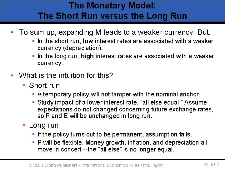
The Monetary Model: The Short Run versus the Long Run • To sum up, expanding M leads to a weaker currency. But: § In the short run, low interest rates are associated with a weaker currency (depreciation). § In the long run, high interest rates are associated with a weaker currency. • What is the intuition for this? w Short run § A temporary policy will not tamper with the nominal anchor. § Study impact of a lower interest rate, “all else equal. ” Assume expectations do not changed concerning future exchange rates, so P and E will be unchanged in long run. w Long run § If the policy turns out to be permanent, assumption fails. § P will be flexible. Money growth, inflation, and depreciation all move in concert—the “all else” is no longer equal. © 2008 Worth Publishers ▪ International Economics ▪ Feenstra/Taylor 22 of 97

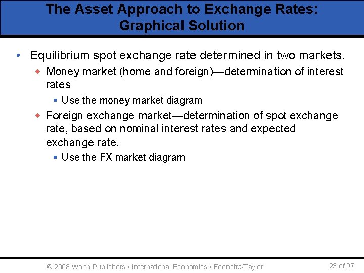
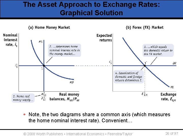
The Asset Approach to Exchange Rates: Graphical Solution • Equilibrium spot exchange rate determined in two markets. w Money market (home and foreign)—determination of interest rates § Use the money market diagram w Foreign exchange market—determination of spot exchange rate, based on nominal interest rates and expected exchange rate. § Use the FX market diagram © 2008 Worth Publishers ▪ International Economics ▪ Feenstra/Taylor 23 of 97

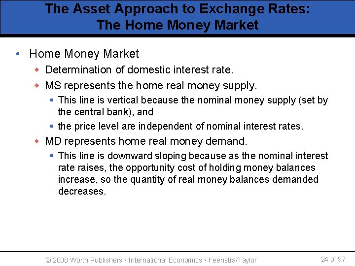
The Asset Approach to Exchange Rates: The Home Money Market • Home Money Market w Determination of domestic interest rate. w MS represents the home real money supply. § This line is vertical because the nominal money supply (set by the central bank), and § the price level are independent of nominal interest rates. w MD represents home real money demand. § This line is downward sloping because as the nominal interest rate raises, the opportunity cost of holding money balances increase, so the quantity of real money balances demanded decreases. © 2008 Worth Publishers ▪ International Economics ▪ Feenstra/Taylor 24 of 97

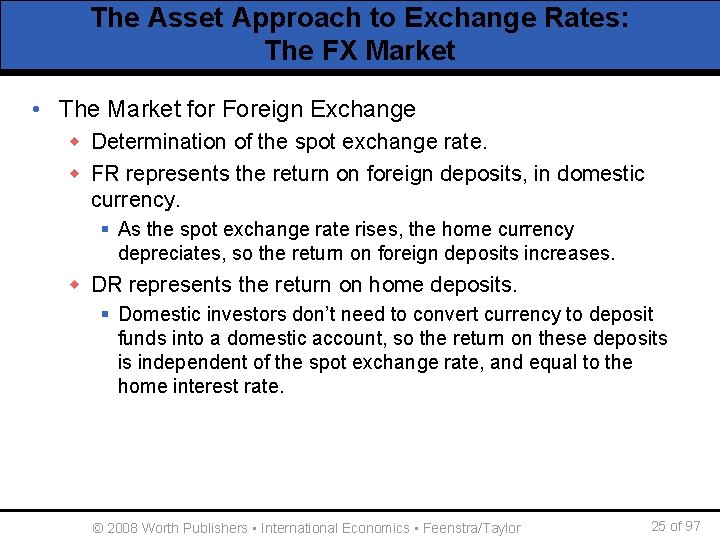
The Asset Approach to Exchange Rates: The FX Market • The Market for Foreign Exchange w Determination of the spot exchange rate. w FR represents the return on foreign deposits, in domestic currency. § As the spot exchange rate rises, the home currency depreciates, so the return on foreign deposits increases. w DR represents the return on home deposits. § Domestic investors don’t need to convert currency to deposit funds into a domestic account, so the return on these deposits is independent of the spot exchange rate, and equal to the home interest rate. © 2008 Worth Publishers ▪ International Economics ▪ Feenstra/Taylor 25 of 97

The Asset Approach to Exchange Rates: Graphical Solution w Note, the two diagrams share a common axis (which measures the home nominal interest rate). Convenient… © 2008 Worth Publishers ▪ International Economics ▪ Feenstra/Taylor 26 of 97

The Asset Approach to Exchange Rates: Capital Mobility is Crucial • This model of exchange rate determination hinges on arbitrage. w The UIP condition, and therefore the intersection of DR and FR being an equilibrium, relies on arbitrage. w If a country imposes capital controls, then investors’ ability to move funds may be diminished or eliminated. w The presence of capital controls may mean that the domestic and foreign returns will not be equal. w Model not well suited for situations with capital controls. © 2008 Worth Publishers ▪ International Economics ▪ Feenstra/Taylor 27 of 97

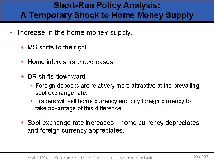
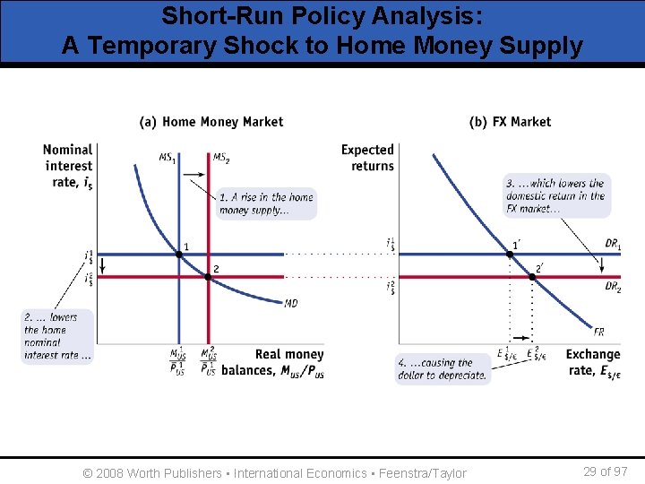
Short-Run Policy Analysis: A Temporary Shock to Home Money Supply • Increase in the home money supply. w MS shifts to the right. w Home interest rate decreases. w DR shifts downward. § Foreign deposits are relatively more attractive at the prevailing spot exchange rate. § Traders will sell home currency and buy foreign currency to take advantage of this difference. w Spot exchange rate increases—home currency depreciates and foreign currency appreciates. © 2008 Worth Publishers ▪ International Economics ▪ Feenstra/Taylor 28 of 97

Short-Run Policy Analysis: A Temporary Shock to Home Money Supply © 2008 Worth Publishers ▪ International Economics ▪ Feenstra/Taylor 29 of 97

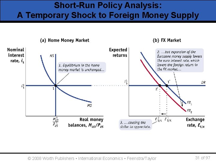
Short-Run Policy Analysis: A Temporary Shock to Foreign Money Supply • Increase in the foreign money supply, M. w Foreign interest rate decreases. w FR shifts downward. § Foreign deposits are relatively less attractive at the prevailing spot exchange rate. § Traders will buy home currency and sell foreign currency to take advantage of this difference. w Spot exchange rate decreases—home currency appreciates and foreign currency depreciates © 2008 Worth Publishers ▪ International Economics ▪ Feenstra/Taylor 30 of 97

Short-Run Policy Analysis: A Temporary Shock to Foreign Money Supply © 2008 Worth Publishers ▪ International Economics ▪ Feenstra/Taylor 31 of 97

The Rise and Fall of the Dollar, 1999– 2004 APPLICATION • During the 1990 s, many countries followed monetary policies that used long-run nominal anchors. w While the European Central bank has an explicit inflation target, the Federal Reserve uses an implicit one. w According to the Fisher effect, nominal anchoring should keep the inflation differentials between countries constant (since the inflation rates in each region are constant). • In the short run, policy makers may deviate from these long-run anchors, in pursuit of other macroeconomic objectives. © 2008 Worth Publishers ▪ International Economics ▪ Feenstra/Taylor 32 of 97

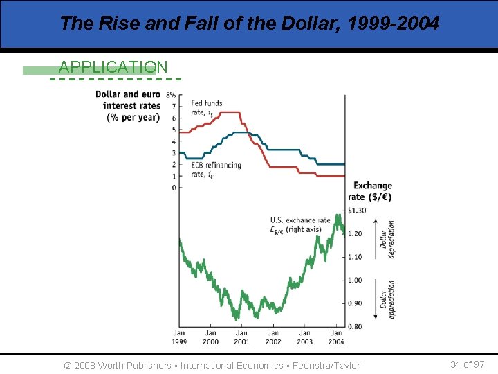
The Rise and Fall of the Dollar, 1999 -2004 APPLICATION § 1999 -2000 § Fed raised interest rates faster and higher than ECB. § 2000 -2002 § Fed lowered interest rates aggressively vs. the ECB, in response to recession and 9/11. § Interest differential falls and then changes sign. § 2002 -2004 § Fed funds rate pushed down further and still well below ECB rate. § What does our model predict for the $/€ exchange rate? © 2008 Worth Publishers ▪ International Economics ▪ Feenstra/Taylor 33 of 97

The Rise and Fall of the Dollar, 1999 -2004 APPLICATION © 2008 Worth Publishers ▪ International Economics ▪ Feenstra/Taylor 34 of 97

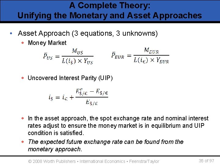
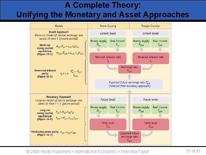
A Complete Theory: Unifying the Monetary and Asset Approaches • Asset Approach (3 equations, 3 unknowns) w Money Market w Uncovered Interest Parity (UIP) w In the asset approach, the spot exchange rate and nominal interest rates adjust to ensure the money market is in equilibrium and UIP condition is satisfied. w The expected future exchange rate can be found from the monetary approach. © 2008 Worth Publishers ▪ International Economics ▪ Feenstra/Taylor 35 of 97

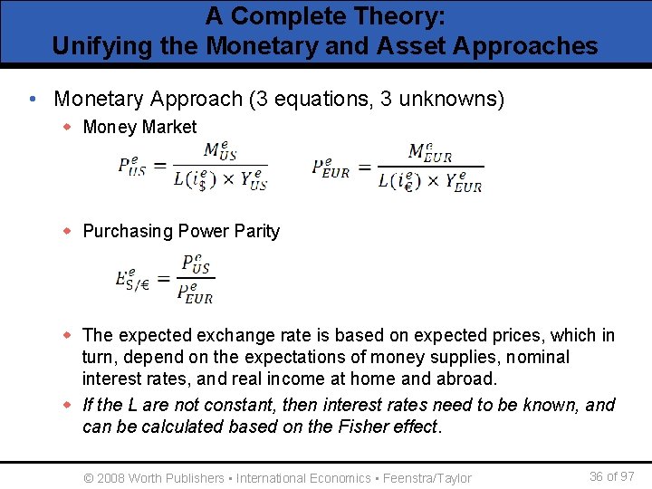
A Complete Theory: Unifying the Monetary and Asset Approaches • Monetary Approach (3 equations, 3 unknowns) w Money Market w Purchasing Power Parity w The expected exchange rate is based on expected prices, which in turn, depend on the expectations of money supplies, nominal interest rates, and real income at home and abroad. w If the L are not constant, then interest rates need to be known, and can be calculated based on the Fisher effect. © 2008 Worth Publishers ▪ International Economics ▪ Feenstra/Taylor 36 of 97

A Complete Theory: Unifying the Monetary and Asset Approaches © 2008 Worth Publishers ▪ International Economics ▪ Feenstra/Taylor 37 of 97

Confessions of a Forex Trader SIDE BAR • Three basic strategies forecasting exchange rates. 1. Economic fundamentals. Investor assumes that exchange rates behave according to economic fundamentals, such as the money supply, price level, and real income. 2. Politics. Factors such as war influence investors’ perception of risk, influencing their forecasts of the exchange rate. 3. Technical methods. This approach relies on statistical methods to predict exchange rate movements, often independent of economic fundamentals. © 2008 Worth Publishers ▪ International Economics ▪ Feenstra/Taylor 38 of 97

Confessions of a Forex Trader SIDE BAR • Which one is most common in practice? w Depends on time horizon. § Most investors believe that intraday, very short-run movements in exchange rates are not based on fundamentals. § Over longer time horizons (6 months, 12 months, etc. ), more and more traders believe fundamentals are important. w Based on the survey, news about money, interest rates, and GDP are quickly incorporated into exchange rate forecasts. © 2008 Worth Publishers ▪ International Economics ▪ Feenstra/Taylor 39 of 97

Long-Run Policy Analysis • Our model can be used for analysis of short run policy experiments. w Key assumption: Temporary policy. w This presumes expected exchange rate is unchanged. w Ignores the long-run building blocks. • The model can be used for long-run analysis as well. w Study permanent monetary policy shocks. w This implies expected exchange rate changes according to the monetary model. § The expected exchange rate changes in the short run, based on long-run forecasts from the monetary model. w Uses all of the building blocks, long run and short run. © 2008 Worth Publishers ▪ International Economics ▪ Feenstra/Taylor 40 of 97

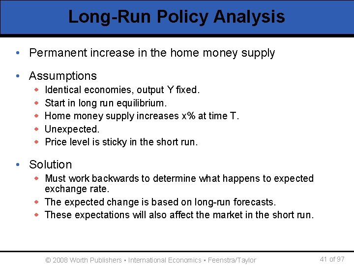
Long-Run Policy Analysis • Permanent increase in the home money supply • Assumptions w w w Identical economies, output Y fixed. Start in long run equilibrium. Home money supply increases x% at time T. Unexpected. Price level is sticky in the short run. • Solution w Must work backwards to determine what happens to expected exchange rate. w The expected change is based on long-run forecasts. w These expectations will also affect the market in the short run. © 2008 Worth Publishers ▪ International Economics ▪ Feenstra/Taylor 41 of 97

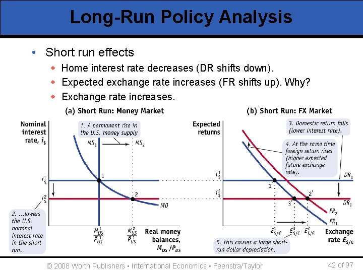
Long-Run Policy Analysis • Short run effects w Home interest rate decreases (DR shifts down). w Expected exchange rate increases (FR shifts up). Why? w Exchange rate increases. © 2008 Worth Publishers ▪ International Economics ▪ Feenstra/Taylor 42 of 97

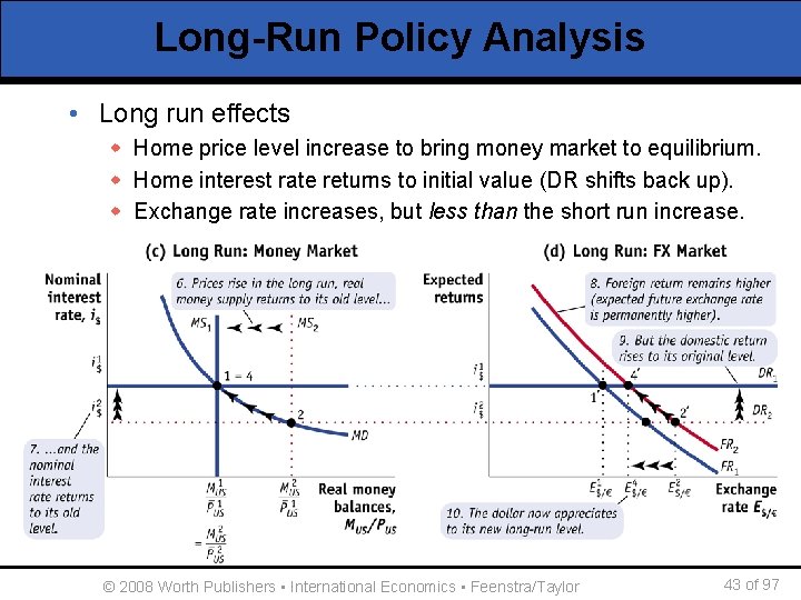
Long-Run Policy Analysis • Long run effects w Home price level increase to bring money market to equilibrium. w Home interest rate returns to initial value (DR shifts back up). w Exchange rate increases, but less than the short run increase. © 2008 Worth Publishers ▪ International Economics ▪ Feenstra/Taylor 43 of 97

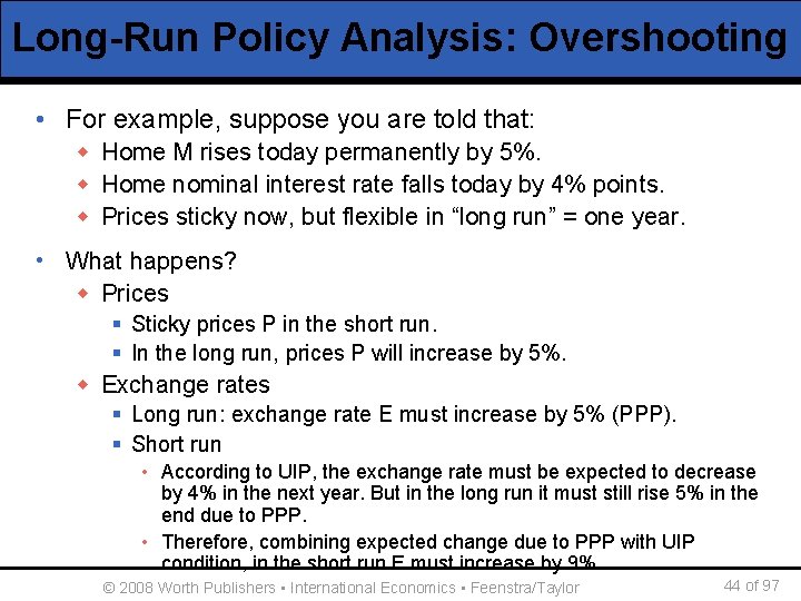
Long-Run Policy Analysis: Overshooting • For example, suppose you are told that: w Home M rises today permanently by 5%. w Home nominal interest rate falls today by 4% points. w Prices sticky now, but flexible in “long run” = one year. • What happens? w Prices § Sticky prices P in the short run. § In the long run, prices P will increase by 5%. w Exchange rates § Long run: exchange rate E must increase by 5% (PPP). § Short run • According to UIP, the exchange rate must be expected to decrease by 4% in the next year. But in the long run it must still rise 5% in the end due to PPP. • Therefore, combining expected change due to PPP with UIP condition, in the short run E must increase by 9%. © 2008 Worth Publishers ▪ International Economics ▪ Feenstra/Taylor 44 of 97

Long-Run Policy Analysis: Overshooting • The exchange rate E overshoots its long run equilibrium after a permanent change in the money supply. Why? w Short run: exchange rate changes for two reasons. § The change in the money market (source of the initial shock) § The effect of this change on exchange rate expectations. § There are two reasons why investors will prefer foreign deposits following an increase in the home money supply. w Long run: nominal interest rate returns to initial value. § The change in exchange rate expectations remain, consistent with a long-run change predicted by PPP. § There is only one reason why investors prefer foreign deposits. © 2008 Worth Publishers ▪ International Economics ▪ Feenstra/Taylor 45 of 97

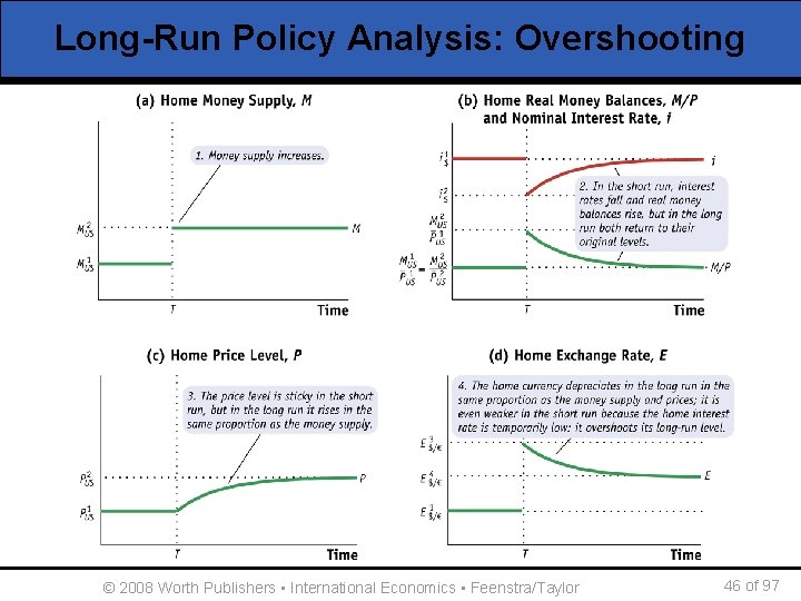
Long-Run Policy Analysis: Overshooting © 2008 Worth Publishers ▪ International Economics ▪ Feenstra/Taylor 46 of 97

Long-Run Policy Analysis: Overshooting • From the figure, we observe how overshooting works. w Money supply § Short run: jumps up to new level. § Long run: remains at new level permanently. w Price level § Short run: no change (assumed to be fixed). § Long run: gradually increases to match the increase in the money supply. w Real money supply § Short run: jumps up with increase in money supply. § Long run: gradually decreases with rising prices. © 2008 Worth Publishers ▪ International Economics ▪ Feenstra/Taylor 47 of 97

Long-Run Policy Analysis: Overshooting • From Figure 15 -13, continued w Nominal interest rate § Short run: jumps down with increase in real money supply. § Long run: gradually increases as real money supply falls. w Exchange rate § Short run: jumps up with decrease in nominal interest rate AND increase in expected exchange rate. § Long run: gradually decreases with rising nominal interest rate. Levels off at a rate above the initial value. © 2008 Worth Publishers ▪ International Economics ▪ Feenstra/Taylor 48 of 97

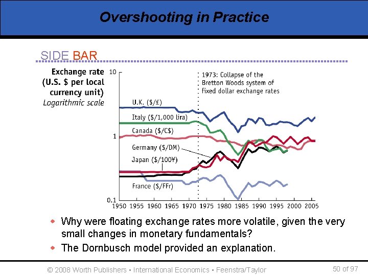
Overshooting in Practice SIDE BAR • Permanent changes in the money supply lead to exchange rate overshooting. w The exchange rate is more volatile than the general monetary model would predict w Result discovered in 1970 s by distinguished economist Rudiger Dornbusch (1942 -2002) • Why this matters in practice. w In the 1970 s the system fixed exchange rates (of the “Bretton Woods system”) collapsed. w Highlights the importance of the nominal anchor. § Under Bretton Woods, countries used an exchange rate target. © 2008 Worth Publishers ▪ International Economics ▪ Feenstra/Taylor 49 of 97

Overshooting in Practice SIDE BAR w Why were floating exchange rates more volatile, given the very small changes in monetary fundamentals? w The Dornbusch model provided an explanation. © 2008 Worth Publishers ▪ International Economics ▪ Feenstra/Taylor 50 of 97

Bernanke’s Bold Move APPLICATION • In the model, changes in the money supply are unexpected. • We studied a simplified time horizon. w In reality, there are significant differences between the interest rate that policy makers control and the ones that matter for investment decisions. w For example, the Federal Reserve and the ECB control an overnight interest rate. w The overnight rate may change several times each year. © 2008 Worth Publishers ▪ International Economics ▪ Feenstra/Taylor 51 of 97

Bernanke’s Bold Move APPLICATION • Investors may anticipate policy moves, so that when the central bank implements the changes, they have no effect on investors’ decisions, or on longer-term rates. • If key economic indicators suggest no clear policy action, then there will be more uncertainty about the central bank’s next move. w When such a policy “surprise” occurs we have a truly unexpected policy change of the kind we assume in our model. © 2008 Worth Publishers ▪ International Economics ▪ Feenstra/Taylor 52 of 97

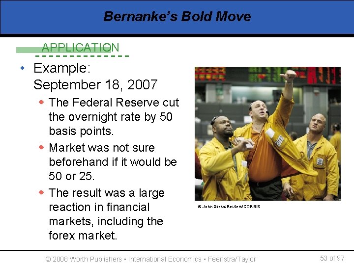
Bernanke’s Bold Move APPLICATION • Example: September 18, 2007 w The Federal Reserve cut the overnight rate by 50 basis points. w Market was not sure beforehand if it would be 50 or 25. w The result was a large reaction in financial markets, including the forex market. © John Gress/Reuters/CORBIS © 2008 Worth Publishers ▪ International Economics ▪ Feenstra/Taylor 53 of 97

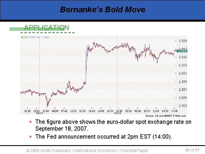
Bernanke’s Bold Move APPLICATION Source: XE. com © 2007 FXtrek. com w The figure above shows the euro-dollar spot exchange rate on September 18, 2007. w The Fed announcement occurred at 2 pm EST (14: 00). © 2008 Worth Publishers ▪ International Economics ▪ Feenstra/Taylor 54 of 97

Bernanke’s Bold Move APPLICATION • Lessons w The Federal Reserve behaved more aggressively than expected. This led to a decrease in interest rates at all maturities up to one year. w The Federal Reserve’s policy might have signaled a shift toward tolerating higher inflation rates in the long run. § From our model, this means that the U. S. dollar is expected to depreciate in the long run. § Also, we know this move would lead to overshooting. The dollar would depreciate more in the short run than in the long run. © 2008 Worth Publishers ▪ International Economics ▪ Feenstra/Taylor 55 of 97

What is a Fixed Exchange Rate Regime? • Consider the case of a fixed exchange rate with a hard peg or narrow bands, without capital controls. w In this case, the government must engage in foreign exchange market intervention to control the value of the currency. w The central bank is responsible for these interventions, through buying and selling foreign currency, in order to keep the exchange rate fixed. w The central bank will manipulate the home money supply, in order to maintain the fixed exchange rate. © 2008 Worth Publishers ▪ International Economics ▪ Feenstra/Taylor 56 of 97

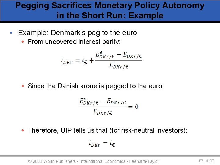
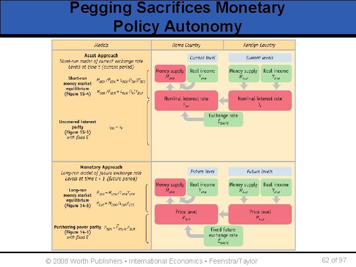
Pegging Sacrifices Monetary Policy Autonomy in the Short Run: Example • Example: Denmark’s peg to the euro w From uncovered interest parity: w Since the Danish krone is pegged to the euro: w Therefore, UIP tells us that (for risk-neutral investors): © 2008 Worth Publishers ▪ International Economics ▪ Feenstra/Taylor 57 of 97

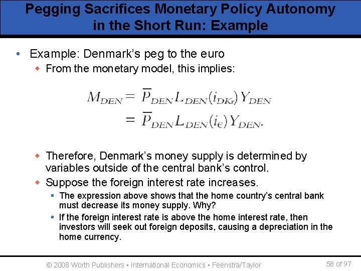
Pegging Sacrifices Monetary Policy Autonomy in the Short Run: Example • Example: Denmark’s peg to the euro w From the monetary model, this implies: w Therefore, Denmark’s money supply is determined by variables outside of the central bank’s control. w Suppose the foreign interest rate increases. § The expression above shows that the home country’s central bank must decrease its money supply. Why? § If the foreign interest rate is above the home interest rate, then investors will seek out foreign deposits, causing a depreciation in the home currency. © 2008 Worth Publishers ▪ International Economics ▪ Feenstra/Taylor 58 of 97

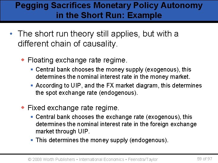
Pegging Sacrifices Monetary Policy Autonomy in the Short Run: Example • The short run theory still applies, but with a different chain of causality. w Floating exchange rate regime. § Central bank chooses the money supply (exogenous), this determines the nominal interest rate in the money market. § According to UIP, and the FX market diagram, this determines the spot exchange rate (endogenous). w Fixed exchange rate regime. § Central bank chooses the exchange rate (exogenous), this determines the nominal interest rate in the foreign exchange market through UIP. § This determines the money supply (endogenous). © 2008 Worth Publishers ▪ International Economics ▪ Feenstra/Taylor 59 of 97

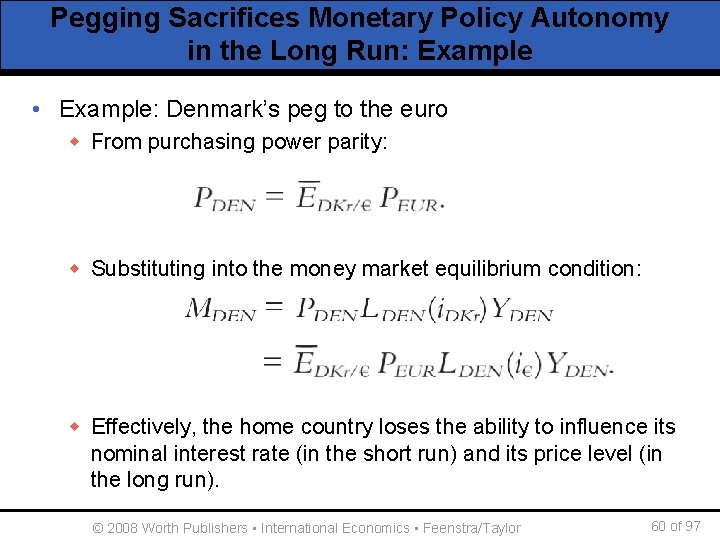
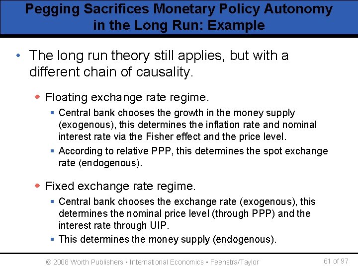
Pegging Sacrifices Monetary Policy Autonomy in the Long Run: Example • Example: Denmark’s peg to the euro w From purchasing power parity: w Substituting into the money market equilibrium condition: w Effectively, the home country loses the ability to influence its nominal interest rate (in the short run) and its price level (in the long run). © 2008 Worth Publishers ▪ International Economics ▪ Feenstra/Taylor 60 of 97

Pegging Sacrifices Monetary Policy Autonomy in the Long Run: Example • The long run theory still applies, but with a different chain of causality. w Floating exchange rate regime. § Central bank chooses the growth in the money supply (exogenous), this determines the inflation rate and nominal interest rate via the Fisher effect and the price level. § According to relative PPP, this determines the spot exchange rate (endogenous). w Fixed exchange rate regime. § Central bank chooses the exchange rate (exogenous), this determines the nominal price level (through PPP) and the interest rate through UIP. § This determines the money supply (endogenous). © 2008 Worth Publishers ▪ International Economics ▪ Feenstra/Taylor 61 of 97

Pegging Sacrifices Monetary Policy Autonomy © 2008 Worth Publishers ▪ International Economics ▪ Feenstra/Taylor 62 of 97

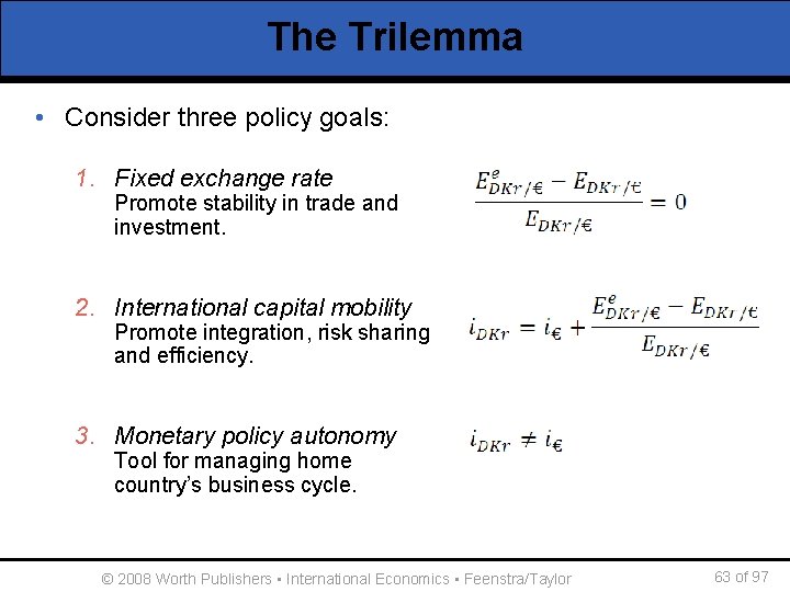
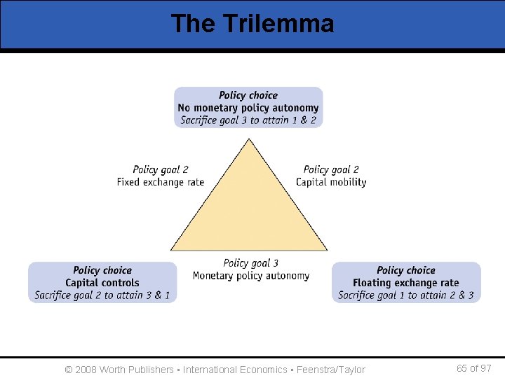
The Trilemma • Consider three policy goals: 1. Fixed exchange rate Promote stability in trade and investment. 2. International capital mobility Promote integration, risk sharing and efficiency. 3. Monetary policy autonomy Tool for managing home country’s business cycle. © 2008 Worth Publishers ▪ International Economics ▪ Feenstra/Taylor 63 of 97

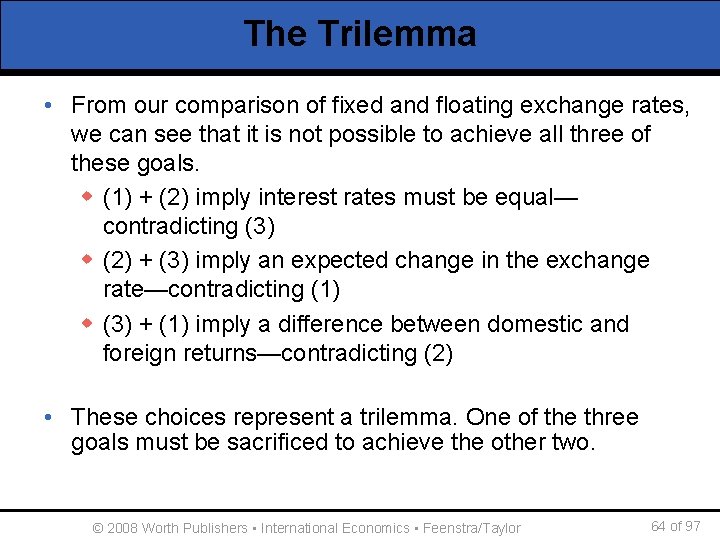
The Trilemma • From our comparison of fixed and floating exchange rates, we can see that it is not possible to achieve all three of these goals. w (1) + (2) imply interest rates must be equal— contradicting (3) w (2) + (3) imply an expected change in the exchange rate—contradicting (1) w (3) + (1) imply a difference between domestic and foreign returns—contradicting (2) • These choices represent a trilemma. One of the three goals must be sacrificed to achieve the other two. © 2008 Worth Publishers ▪ International Economics ▪ Feenstra/Taylor 64 of 97

The Trilemma © 2008 Worth Publishers ▪ International Economics ▪ Feenstra/Taylor 65 of 97

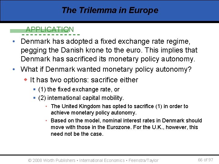
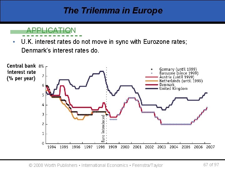
The Trilemma in Europe APPLICATION • Denmark has adopted a fixed exchange rate regime, pegging the Danish krone to the euro. This implies that Denmark has sacrificed its monetary policy autonomy. • What if Denmark wanted monetary policy autonomy? w It has two options: sacrifice either § (1) the fixed exchange rate, or § (2) international capital mobility. • The United Kingdom has opted to sacrifice (1) in order to achieve monetary policy autonomy. • Based on the model, nominal interest rates in Denmark should move with those in the Eurozone. For the U. K. , however, this need not be the case. © 2008 Worth Publishers ▪ International Economics ▪ Feenstra/Taylor 66 of 97

The Trilemma in Europe APPLICATION • U. K. interest rates do not move in sync with Eurozone rates; Denmark’s interest rates do. © 2008 Worth Publishers ▪ International Economics ▪ Feenstra/Taylor 67 of 97

News and the Foreign Exchange Market APPLICATION • During wartime, there is greater likelihood of observing dramatic changes in the exchange rate. Why? w Governments often finance war through printing money, generating inflation. w The uncertainty associated with war allow for dramatic changes in money demand, as there is a risk that the currency may be converted into another currency unit, or eliminated altogether. © 2008 Worth Publishers ▪ International Economics ▪ Feenstra/Taylor 68 of 97

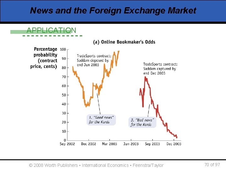
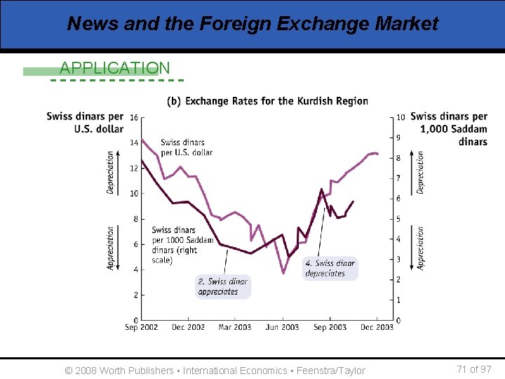
News and the Foreign Exchange Market APPLICATION • The Iraq War, 2002– 03 w In 2003 a U. S. -led coalition invaded Iraq, intent on ending the government of Saddam Hussein. w At the time, two currencies in use: “Swiss” dinars in the north (Kurdish region) and “Saddam” dinars in the south. § Eventually, currency reform established a new dinar, with the old currency units convertible during the transition. w The exchange rate fluctuates as expected. As hostilities between the U. S. and Iraq escalated in 2002 and 2003, the Swiss dinar appreciated (“good news” for Kurds). w After Hussein was deposed and went into hiding, political instability escalated, and Hussein could not be found for a long time. The Swiss dinar then depreciated (“bad news” for the Kurds). © 2008 Worth Publishers ▪ International Economics ▪ Feenstra/Taylor 69 of 97

News and the Foreign Exchange Market APPLICATION © 2008 Worth Publishers ▪ International Economics ▪ Feenstra/Taylor 70 of 97

News and the Foreign Exchange Market APPLICATION © 2008 Worth Publishers ▪ International Economics ▪ Feenstra/Taylor 71 of 97