The statistical analysis of f MRI data Keith

The statistical analysis of f. MRI data Keith Worsley 12, Chuanhong Liao 1, John Aston 123, Jean-Baptiste Poline 4, Gary Duncan 5, Vali Petre 2, Frank Morales 6, Alan Evans 2, Tom Nichols 7, Satoru Hayasaki 7 1 Department of Mathematics and Statistics, Mc. Gill University, 2 Brain Imaging Centre, Montreal Neurological Institute, 3 Imperial College, London, 4 Service Hospitalier Frédéric Joliot, CEA, Orsay, 5 Centre de Recherche en Sciences Neurologiques, Université de Montréal, 6 Cuban Neuroscience Centre 7 University of Michigan

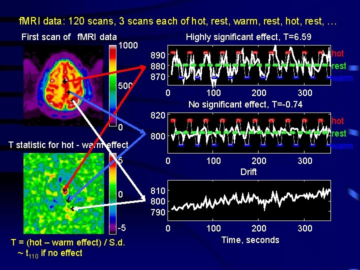
f. MRI data: 120 scans, 3 scans each of hot, rest, warm, rest, hot, rest, … First scan of f. MRI data 1000 500 Highly significant effect, T=6. 59 hot rest warm 890 880 870 0 100 200 300 No significant effect, T=-0. 74 820 0 T statistic for hot - warm effect 800 5 0 -5 T = (hot – warm effect) / S. d. ~ t 110 if no effect hot rest warm 0 100 200 Drift 300 810 800 790 200 Time, seconds 300

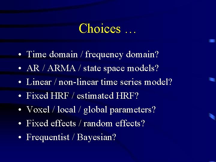
Choices … • • Time domain / frequency domain? AR / ARMA / state space models? Linear / non-linear time series model? Fixed HRF / estimated HRF? Voxel / local / global parameters? Fixed effects / random effects? Frequentist / Bayesian?

More importantly. . . • • Fast execution / slow execution? Matlab / C? Script (batch) / GUI? Lazy / hard working … ? Why not just use SPM? Develop new ideas. . . FMRISTAT: Simple, general, valid, robust, fast analysis of f. MRI data

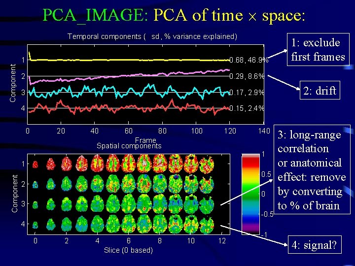
PCA_IMAGE: PCA of time space: Component Temporal components ( sd , % variance explained) 1 0. 68, 46. 9% 2 0. 29, 8. 6% 3 0. 17, 2. 9% 4 0. 15, 2. 4% 0 20 40 60 80 100 120 140 Frame Spatial components 1 Component 1 0. 5 2 0 3 -0. 5 1: exclude first frames 2: drift 3: long-range correlation or anatomical effect: remove by converting to % of brain 4 0 2 4 6 8 Slice (0 based) 10 12 -1 4: signal?

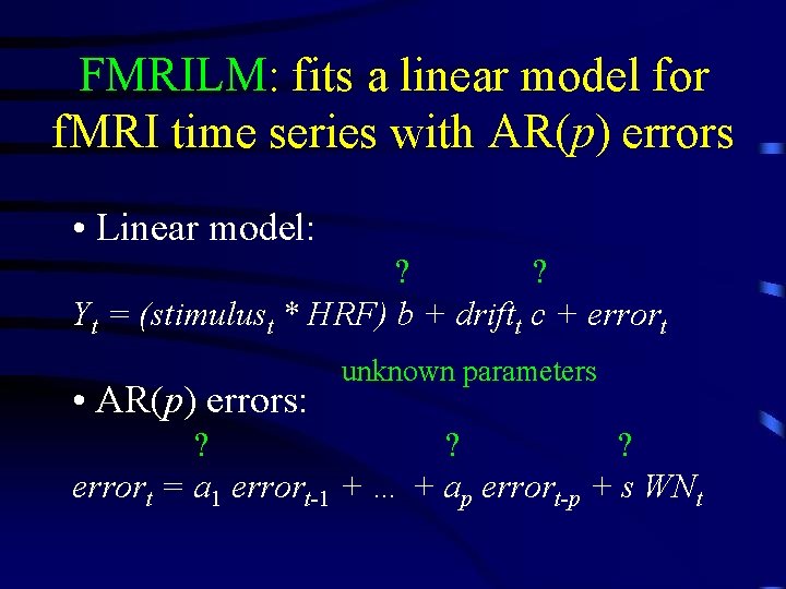
FMRILM: fits a linear model for f. MRI time series with AR(p) errors • Linear model: ? ? Yt = (stimulust * HRF) b + driftt c + errort • AR(p) errors: unknown parameters ? ? ? errort = a 1 errort-1 + … + ap errort-p + s WNt

FMRIDESIGN example: pain perception 1 ho t w ar m 2 Alternating hot and warm stimuli separated by rest (9 seconds each). 0 -1 0 50 100 150 200 250 300 350 Hemodynamic response function: difference of two gamma densities 0. 4 0. 2 0 -0. 2 0 50 Responses = stimuli * HRF, sampled every 3 seconds 2 1 0 -1 0 50 100 150 200 Time, seconds 250 300 350

FMRILM first step: estimate the autocorrelation ? AR(1) model: errort = a 1 errort-1 + s WNt • Fit the linear model using least squares • errort = Yt – fitted Yt • â 1 = Correlation ( errort , errort-1) • Estimating errort’s changes their correlation structure slightly, so â 1 is slightly biased: which_stats = ‘_cor’ Raw autocorrelation Smoothed 12. 4 mm ~ -0. 05 Bias corrected â 1 ~0

Effective df depends on smoothing • Variability in 2 3/2 FWHM acor lowers df dfacor = dfresidual 2 FWHM 2 + 1 • Df depends data 1 1 2 acor(contrast of data)2 on contrast = + • Smoothing acor dfeff dfresidual dfacor brings df back up: Hot stimulus FWHMdata = 8. 79 Hot-warm stimulus ( Residual df = 110 100 Target = 100 df 50 Contrast of data, acor = 0. 61 dfeff 0 0 10 20 30 FWHM = 10. 3 mm FWHMacor ) Residual df = 110 100 Target = 100 df 50 Contrast of data, acor = 0. 79 dfeff 0 0 10 20 30 FWHM = 12. 4 mm FWHMacor

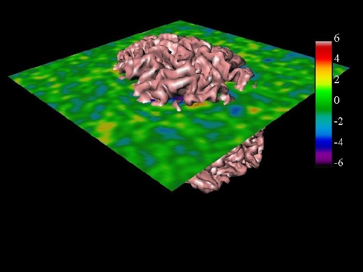
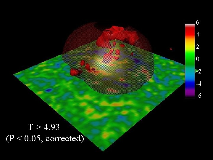
FMRILM second step: refit the linear model Pre-whiten: Yt* = Yt – â 1 Yt-1, then fit using least squares: Hot - warm effect, % ‘_mag_ef’ Sd of effect, % ‘_mag_sd’ 1 0. 25 0. 2 0. 5 0. 15 0 0. 1 -0. 5 0. 05 -1 T = effect / sd, 110 df ‘_mag_t’ 6 4 2 0 -2 -4 -6 0 which_stats = ‘_mag_ef _mag_sd _mag_t’ T > 4. 93 (P < 0. 05, corrected)

Higher order AR model? Try AR(3): ‘_AR’ a 1 a 2 a 3 0. 2 AR(1) seems to be adequate 0. 1 0 No correlation … has little effect on the T statistics: AR(1), df =100 AR(2), df =98 -0. 1 AR(3), df =98 5 0 -5 biases T up ~12% → more false positives

Results from 4 runs on the same subject Run 1 Effect, Ei Run 2 Run 3 Run 4 1 0 ‘_mag_ef’ -1 Sd, Si ‘_mag_sd’ 0. 2 0. 1 0 5 T stat, E i / Si ‘_mag_t’ 0 -5

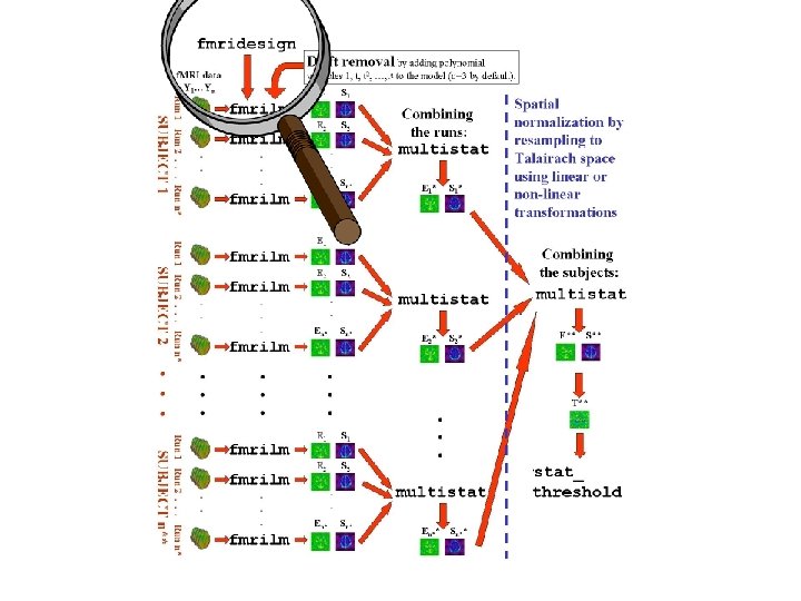
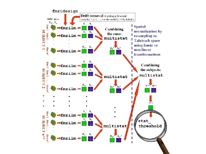
MULTISTAT: mixed effects linear model for combining effects from different runs/sessions/subjects: • Ei = effect for run/session/subject i from • Si = standard error of effect FMRILM • Mixed effects model: ? ? F Ei = covariatesi c + Si WNi + WNi. R } Usually 1, but could add group, treatment, age, sex, . . . ‘Fixed effects’ error, due to variability within the same run Random effect, due to variability from run to run

REML estimation using the EM algorithm • • Slow to converge (10 iterations by default). Stable (maintains estimate ^2 > 0 ), but ^2 biased if 2 (random effect) is small, so: Re-parameterize the variance model: ? 2 2 Var(Ei) = Si + = (Si 2 – minj Sj 2) + ( 2 + minj Sj 2) ? 2 2 = Si* + * ^2 = * ^ 2 – min S 2 (less biased estimate) • j j

Problem: 4 runs, 3 df for random effects sd . . . Run 1 Run 2 Run 3 Run 4 MULTISTAT Effect, Ei 1 0 ‘_mag_ef’ … very noisy sd: -1 0. 2 Sd, Si 0. 1 ‘_mag_sd’ … and T>15. 96 for P<0. 05 (corrected): 0 5 T stat, E i / Si 0 ‘_mag_t’ … so no response is detected … -5

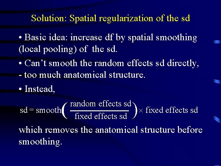
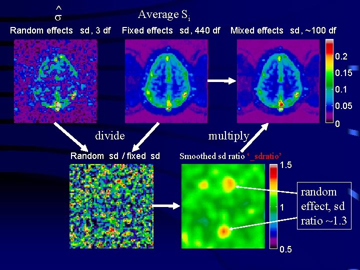
Solution: Spatial regularization of the sd • Basic idea: increase df by spatial smoothing (local pooling) of the sd. • Can’t smooth the random effects sd directly, - too much anatomical structure. • Instead, sd = smooth ) random effects sd fixed effects sd which removes the anatomical structure before smoothing.

^ Average Si Random effects sd , 3 df Fixed effects sd , 440 df Mixed effects sd , ~100 df 0. 2 0. 15 0. 1 0. 05 divide Random sd / fixed sd 0 multiply Smoothed sd ratio ‘_sdratio’ 1. 5 1 0. 5 random effect, sd ratio ~1. 3

Effective df depends on smoothing ( FWHMratio 2 dfratio = dfrandom 2 FWHM 2 + 1 data 1 = 1 + 1 dfeff dfratio dffixed ) 3/2 e. g. dfrandom = 3, dffixed = 4 110 = 440, FWHMdata = 8 mm: fixed effects analysis, dfeff = 440 400 300 dfeff Target = 100 df random effects analysis, dfeff = 3 200 FWHM = 19 mm 100 0 0 20 40 FWHMratio Infinity

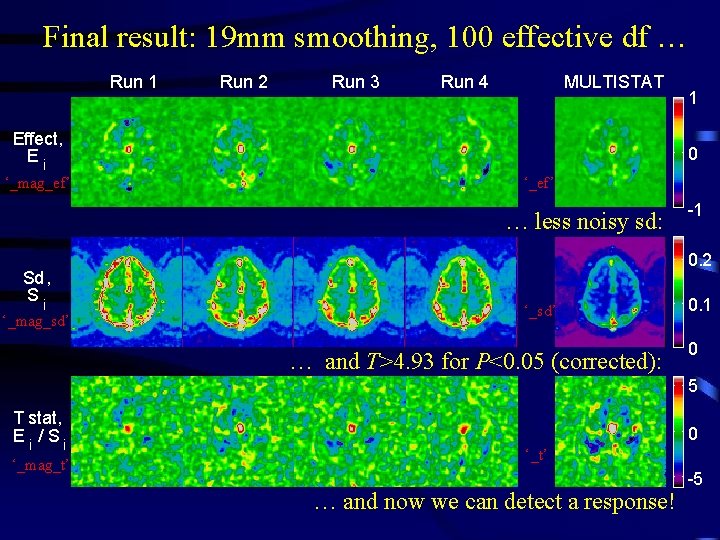
Final result: 19 mm smoothing, 100 effective df … Run 1 Run 2 Run 3 Run 4 MULTISTAT Effect, Ei ‘_mag_ef’ 0 ‘_ef’ … less noisy sd: Sd, Si ‘_mag_sd’ 1 -1 0. 2 ‘_sd’ … and T>4. 93 for P<0. 05 (corrected): 0. 1 0 5 T stat, E i / Si ‘_mag_t’ 0 ‘_t’ … and now we can detect a response! -5

FWHM – the local smoothness of the noise FWHM = voxel size (2 log 2)1/2 (1 – correlation) (If the noise is modeled as white noise smoothed with a Gaussian kernel, this would be its FWHM) 0. 1 Local maximum T = 4. 5 Clusters above t = 3. 0, search volume 0. 1 P value of cluster P value of local max P-values depend on Resels: 0. 08 0. 06 0. 04 0. 02 0 0 Volume Resels = FWHM 3 500 1000 Resels of search volume 0. 08 0. 06 0. 04 0. 02 0 0 0. 5 1 1. 5 Resels of cluster 2 resels = 500

Non-isotropic data (spatially varying FWHM) • f. MRI data is smoother in GM than WM • VBM data is highly non-isotropic • Has little effect on P-values for local maxima (use ‘average’ FWHM inside search region), but • Has a big effect on P-values for spatial extents: smooth regions → big clusters, rough regions → small clusters, so • Replace cluster volume by cluster resels = volume / FWHM 3

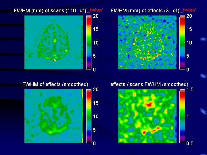
FWHM (mm) of scans (110 df )‘_fwhm’ 20 Resels=1. 90 P=0. 007 Resels=0. 57 P=0. 387 FWHM of effects (smoothed) FWHM (mm) of effects (3 df )‘_fwhm’ 20 15 15 10 10 5 5 0 0 20 effects / scans FWHM (smoothed) 1. 5 15 10 1 5 0 0. 5

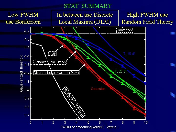
STAT_SUMMARY In between use Discrete Local Maxima (DLM) Low FWHM use Bonferroni High FWHM use Random Field Theory Bonferroni 4. 7 4. 6 True 4. 4 T, 10 df Random Field Theory 4. 3 T, 20 df Discrete Local Maxima (DLM) 4. 2 4. 1 4 Gaussian r nfe Bo Gaussianized threshold 4. 5 ni ro 3. 9 , N es =R 3. 8 els 3. 7 0 1 2 3 4 5 6 7 8 FWHM of smoothing kernel ( voxels ) 9 10

STAT_SUMMARY In between use Discrete Local Maxima (DLM) Low FWHM use Bonferroni High FWHM use Random Field Theory 0. 12 Gaussian T, 20 df T, 10 df 0. 1 Random Field Theory Bonferroni P-value 0. 08 DLM can ½ P-value when FWHM ~3 voxels 0. 06 0. 04 True Discrete Local Maxima 0. 02 Bonferroni , N=Resels 0 0 1 2 3 4 5 6 7 8 FWHM of smoothing kernel ( voxels ) 9 10

STAT_SUMMARY example: single run, hot-warm Detected by BON and DLM but not by RFT Detected by DLM, but not by BON or RFT

T>4. 86

T>4. 86 T > 4. 93 (P < 0. 05, corrected)

T>4. 86 T > 4. 93 (P < 0. 05, corrected)

T>4. 86

Conjunction: Minimum Ti > threshold Minimum of Ti ‘_conj’ For P=0. 05, threshold = 1. 82 Efficiency = 82% Average of Ti ‘_mag_t’ For P=0. 05, threshold = 4. 93

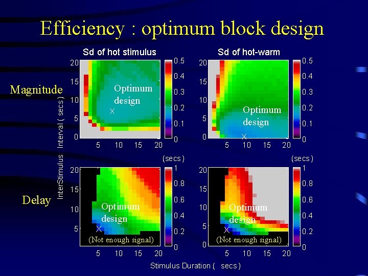
Efficiency : optimum block design Sd of hot stimulus 0. 5 20 Delay Inter. Stimulus Interval ( secs ) Magnitude 0. 4 15 Optimum design 10 0. 2 X 5 0 0. 3 0. 1 5 10 15 20 (secs ) 1 20 0. 8 15 0. 6 Optimum design 10 5 0 0. 4 X (Not enough signal) 5 10 15 0. 2 20 0 Sd of hot-warm 0. 5 20 0. 4 15 0. 3 10 5 0 0. 2 Optimum design X 10 5 15 0. 1 20 (secs ) 1 20 0. 8 15 0 0. 6 Optimum design 10 5 0 0. 4 X (Not enough signal) 5 Stimulus Duration ( secs ) 10 15 0. 2 20 0

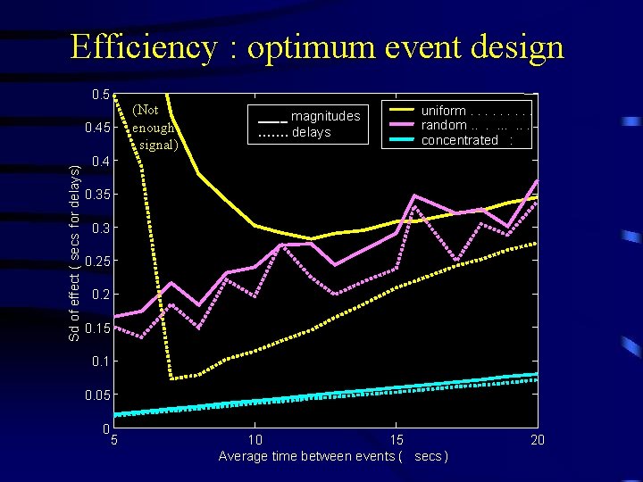
Efficiency : optimum event design 0. 5 Sd of effect ( secs for delays) 0. 45 (Not enough signal) ____ magnitudes ……. delays uniform. . random. . concentrated : 0. 4 0. 35 0. 3 0. 25 0. 2 0. 15 0. 1 0. 05 0 5 10 15 Average time between events ( secs ) 20

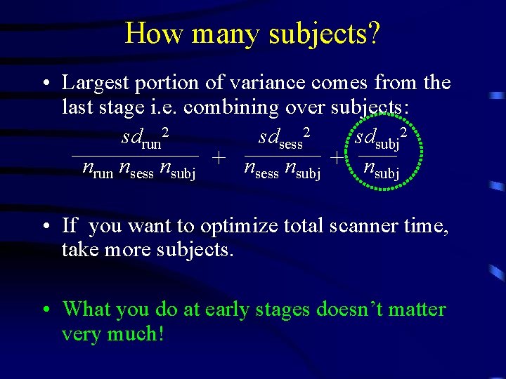
How many subjects? • Largest portion of variance comes from the last stage i. e. combining over subjects: sdrun 2 sdsess 2 sdsubj 2 nrun nsess nsubj + nsubj • If you want to optimize total scanner time, take more subjects. • What you do at early stages doesn’t matter very much!

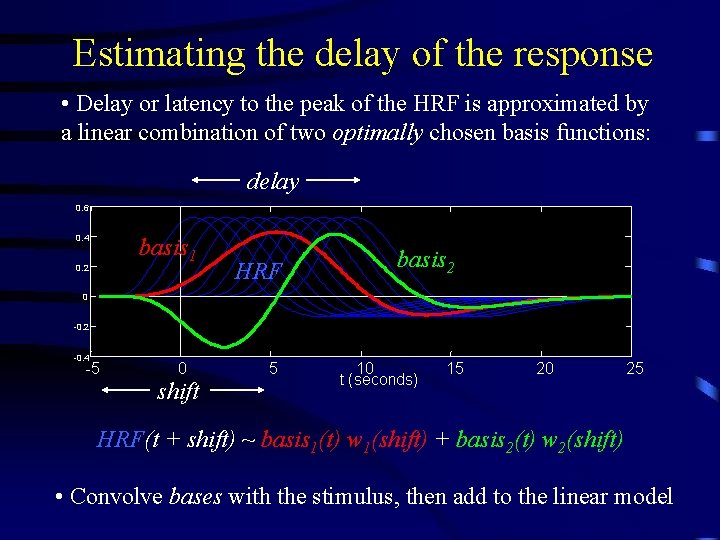
Estimating the delay of the response • Delay or latency to the peak of the HRF is approximated by a linear combination of two optimally chosen basis functions: delay 0. 6 0. 4 basis 1 0. 2 HRF basis 2 0 -0. 2 -0. 4 -5 0 shift 5 10 t (seconds) 15 20 25 HRF(t + shift) ~ basis 1(t) w 1(shift) + basis 2(t) w 2(shift) • Convolve bases with the stimulus, then add to the linear model

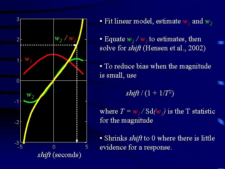
• Fit linear model, estimate w 1 and w 2 3 w 2 / w 1 2 1 • Equate w 2 / w 1 to estimates, then solve for shift (Hensen et al. , 2002) w 1 • To reduce bias when the magnitude is small, use 0 -1 shift / (1 + 1/T 2) w 2 -2 where T = w 1 / Sd(w 1) is the T statistic for the magnitude -3 -5 • Shrinks shift to 0 where there is little evidence for a response. 0 shift (seconds) 5

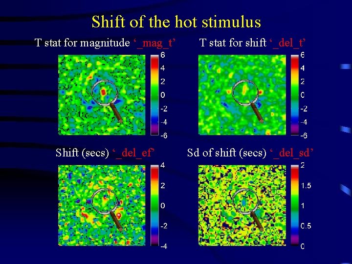
Shift of the hot stimulus T stat for magnitude ‘_mag_t’ T stat for shift ‘_del_t’ Shift (secs) ‘_del_ef’ Sd of shift (secs) ‘_del_sd’

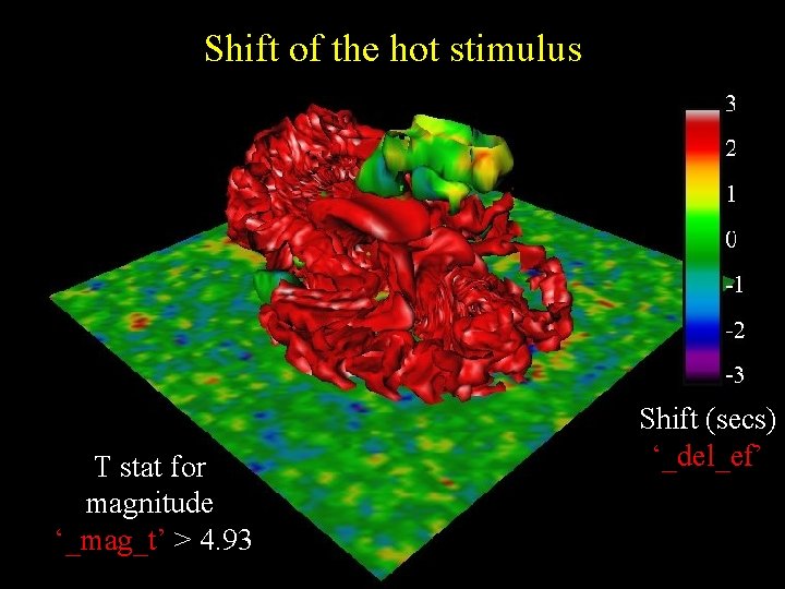
Shift of the hot stimulus T stat for magnitude ‘_mag_t’ T>4 Shift (secs) ‘_del_ef’ ~1 sec T stat for shift ‘_del_t’ T~2 Sd of shift (secs) ‘_del_sd’ +/- 0. 5 sec

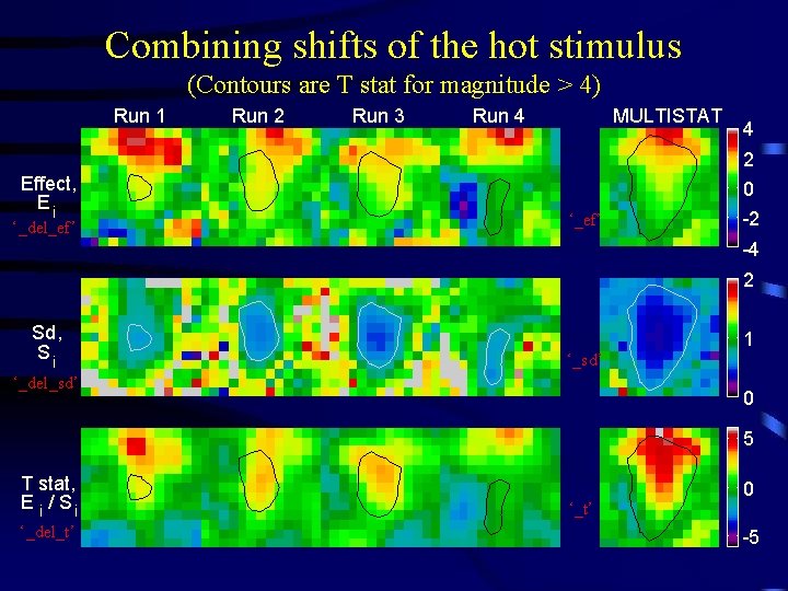
Combining shifts of the hot stimulus (Contours are T stat for magnitude > 4) Run 1 Run 2 Run 3 Run 4 MULTISTAT 4 2 Effect, Ei ‘_del_ef’ 0 ‘_ef’ -2 -4 2 Sd, Si 1 ‘_sd’ ‘_del_sd’ 0 5 T stat, E i / Si ‘_del_t’ ‘_t’ 0 -5

Shift of the hot stimulus T stat for magnitude ‘_mag_t’ > 4. 93 Shift (secs) ‘_del_ef’

Comparison: SPM’ 99: fmristat: • Different slice acquisition times: • Drift removal: • Shifts the model • Temporal correlation: • Estimation of effects: • Rationale: • Random effects: • Map of the delay: • Adds a temporal derivative • Low frequency cosines (flat at the ends) • AR(1), global parameter, bias reduction not necessary • Band pass filter, then least-squares, then correction for temporal correlation • More robust, but lower df • No regularization, low df, no conjuncs • No • Splines (free at the ends) • AR(p), voxel parameters, bias reduction • Pre-whiten, then least squares (no further corrections needed) • More accurate, higher df • Regularization, high df, conjuncs • Yes

References • http: //www. math. mcgill. ca/keith/fmristat • Worsley et al. (2002). A general statistical analysis for f. MRI data. Neuro. Image, 15: 115. • Liao et al. (2002). Estimating the delay of the response in f. MRI data. Neuro. Image, 16: 593 -606.

Functional connectivity • Measured by the correlation between residuals at every pair of voxels (6 D data!) Activation only Voxel 2 ++ + +++ Correlation only Voxel 2 Voxel 1 + • • + ++ Voxel 1 + + Local maxima are larger than all 12 neighbours P-value can be calculated using random field theory Good at detecting focal connectivity, but PCA of residuals x voxels is better at detecting large regions of co-correlated voxels

|Correlations| > 0. 7, P<10 -10 (corrected) First Principal Component > threshold

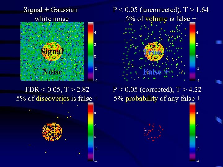
False Discovery Rate (FDR) Benjamini and Hochberg (1995), Journal of the Royal Statistical Society Benjamini and Yekutieli (2001), Annals of Statistics Genovese et al. (2001), Neuro. Image • FDR controls the expected proportion of false positives amongst the discoveries, whereas • Bonferroni / random field theory controls the probability of any false positives • No correction controls the proportion of false positives in the volume

Signal + Gaussian white noise P < 0. 05 (uncorrected), T > 1. 64 5% of volume is false + Signal True + Noise False + FDR < 0. 05, T > 2. 82 5% of discoveries is false + P < 0. 05 (corrected), T > 4. 22 5% probability of any false +

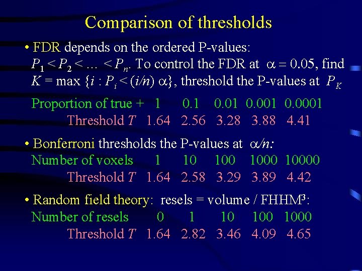
Comparison of thresholds • FDR depends on the ordered P-values: P 1 < P 2 < … < Pn. To control the FDR at a = 0. 05, find K = max {i : Pi < (i/n) a}, threshold the P-values at PK Proportion of true + 1 0. 01 0. 0001 Threshold T 1. 64 2. 56 3. 28 3. 88 4. 41 • Bonferroni thresholds the P-values at a/n: Number of voxels 1 10 10000 Threshold T 1. 64 2. 58 3. 29 3. 89 4. 42 • Random field theory: resels = volume / FHHM 3: Number of resels 0 1 10 1000 Threshold T 1. 64 2. 82 3. 46 4. 09 4. 65

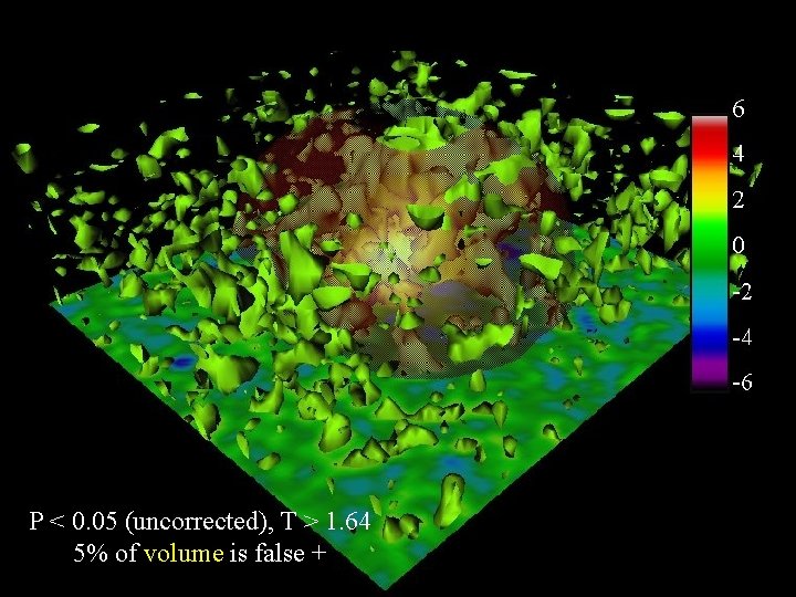
P < 0. 05 (uncorrected), T > 1. 64 5% of volume is false +

FDR < 0. 05, T > 2. 67 5% of discoveries is false +

P < 0. 05 (corrected), T > 4. 93 5% probability of any false +

Random fields and brain mapping Keith Worsley Department of Mathematics and Statistics, Mc. Connell Brain Imaging Centre, Montreal Neurological Institute, Mc. Gill University