On the Statistical Analysis of Dirty Pictures Julian

On the Statistical Analysis of Dirty Pictures Julian Besag 1

Image Processing n Required in a very wide range of practical problems ¨ Computer vision ¨ Computer tomography ¨ Agriculture ¨ Many more… n Picture acquisition techniques are noisy 2

Problem Statement Given a noisy picture n And 2 source of information (assumptions) n ¨A multivariate record for each pixel ¨ Pixels close together tend to be alike n Reconstruct the true scene 3

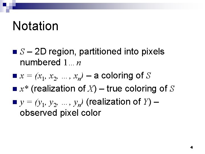
Notation S – 2 D region, partitioned into pixels numbered 1…n n x = (x 1, x 2, …, xn) – a coloring of S n x* (realization of X) – true coloring of S n y = (y 1, y 2, …, yn) (realization of Y) – observed pixel color n 4

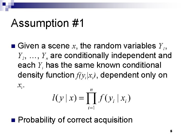
Assumption #1 n Given a scene x, the random variables Y 1, Y 2, …, Yn are conditionally independent and each Yi has the same known conditional density function f(yi|xi), dependent only on x i. n Probability of correct acquisition 5

Assumption #2 n The true coloring x* is a realization of a locally dependant Markov random field with specified distribution {p(x)} 6

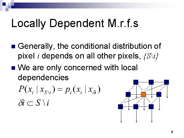
Locally Dependent M. r. f. s Generally, the conditional distribution of pixel i depends on all other pixels, {Si} n We are only concerned with local dependencies n 7

Previous Methodology Maximum Probability Estimation n Classification by Maximum Marginal Probabilities n 8

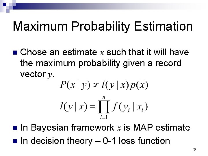
Maximum Probability Estimation n Chose an estimate x such that it will have the maximum probability given a record vector y. In Bayesian framework x is MAP estimate n In decision theory – 0 -1 loss function n 9

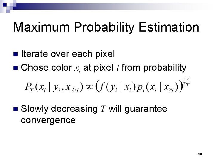
Maximum Probability Estimation Iterate over each pixel n Chose color xi at pixel i from probability n n Slowly decreasing T will guarantee convergence 10

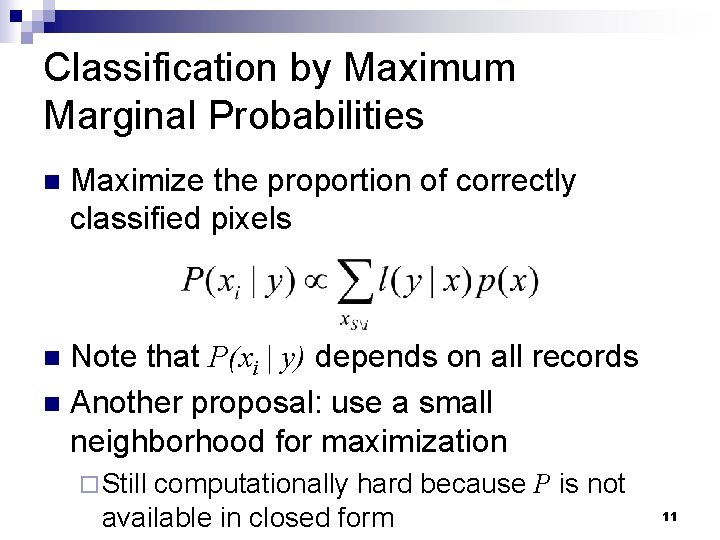
Classification by Maximum Marginal Probabilities n Maximize the proportion of correctly classified pixels Note that P(xi | y) depends on all records n Another proposal: use a small neighborhood for maximization n ¨ Still computationally hard because P is not available in closed form 11

Problems n Large scale effects ¨ Favors n scenes of single color Computationally expensive 12

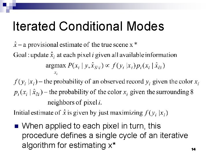
Estimation by Iterated Conditional Modes n n The previously discussed methods have enormous computational demands, and undesirable large-scale properties. We want a faster method with good large-scale properties. 13

Iterated Conditional Modes n When applied to each pixel in turn, this procedure defines a single cycle of an iterative algorithm for estimating x* 14

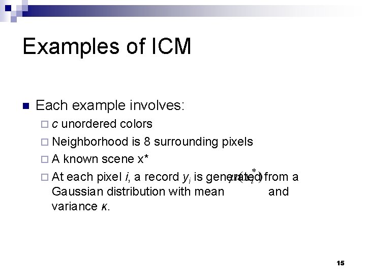
Examples of ICM n Each example involves: ¨c unordered colors ¨ Neighborhood is 8 surrounding pixels ¨ A known scene x* ¨ At each pixel i, a record yi is generated from a Gaussian distribution with mean and variance κ. 15

The hillclimbing update step 16

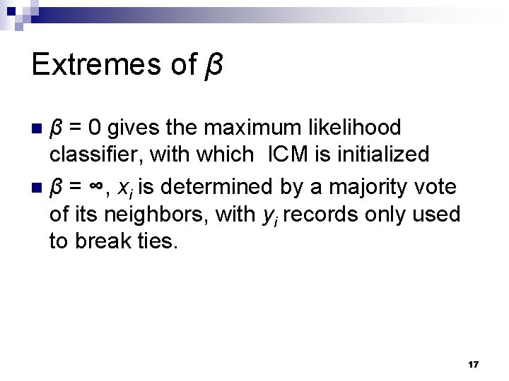
Extremes of β β = 0 gives the maximum likelihood classifier, with which ICM is initialized n β = ∞, xi is determined by a majority vote of its neighbors, with yi records only used to break ties. n 17

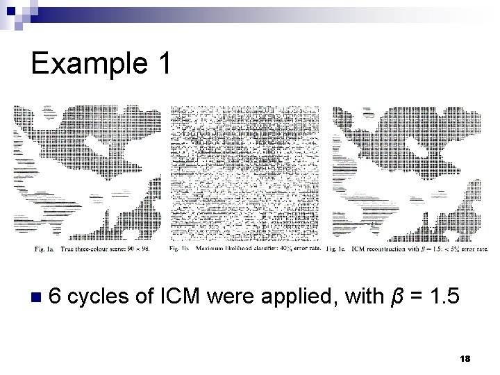
Example 1 n 6 cycles of ICM were applied, with β = 1. 5 18

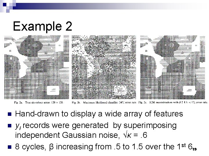
Example 2 n n n Hand-drawn to display a wide array of features yi records were generated by superimposing independent Gaussian noise, √κ =. 6 8 cycles, β increasing from. 5 to 1. 5 over the 1 st 619

Models for the true scene Most of the material here is speculative, a topic for future research n There are many kinds of images possessing special structures in the true scene. n What we have seen so far in the examples are discrete ordered colors. n 20

Examples of special types of images n Unordered colors ¨ These are generally codes for some other attribute, such as crop identities n Excluded adjacencies ¨ It may be known that certain colors cannot appear on neighboring pixels in the true scene. 21

More special cases… n Grey-level scenes ¨ Colors may have a natural ordering, such as intensity. The authors did not have the computing equipment to process, display, and experiment with 256 grey levels. n Continuous intensities ¨ {p(x)} is a Gaussian M. r. f. with zero mean 22

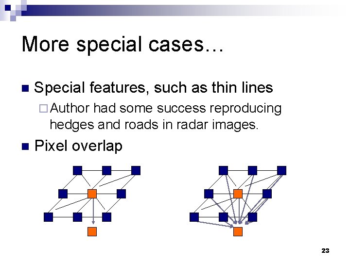
More special cases… n Special features, such as thin lines ¨ Author had some success reproducing hedges and roads in radar images. n Pixel overlap 23

Parameter Estimation This may be computationally expensive n This is often unnecessary n We may need to estimate θ in l(y|x; θ) n ¨ Learn n how records result from true scenes. And we may need to estimate Φ in p(x; Φ) ¨ Learn probabilities of true scenes. 24

Parameter Estimation, cont. n n Estimation from training data Estimation during ICM 25

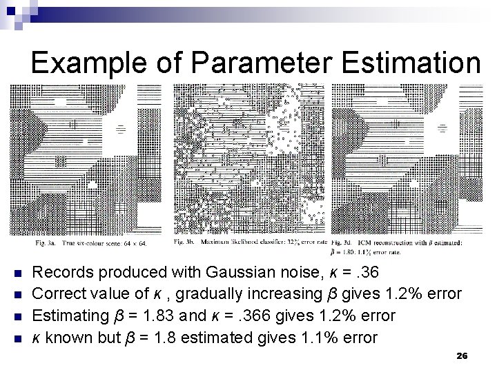
Example of Parameter Estimation n n Records produced with Gaussian noise, κ =. 36 Correct value of κ , gradually increasing β gives 1. 2% error Estimating β = 1. 83 and κ =. 366 gives 1. 2% error κ known but β = 1. 8 estimated gives 1. 1% error 26

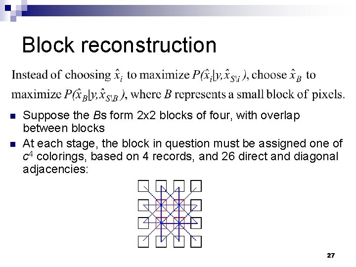
Block reconstruction n n Suppose the Bs form 2 x 2 blocks of four, with overlap between blocks At each stage, the block in question must be assigned one of c 4 colorings, based on 4 records, and 26 direct and diagonal adjacencies: 27

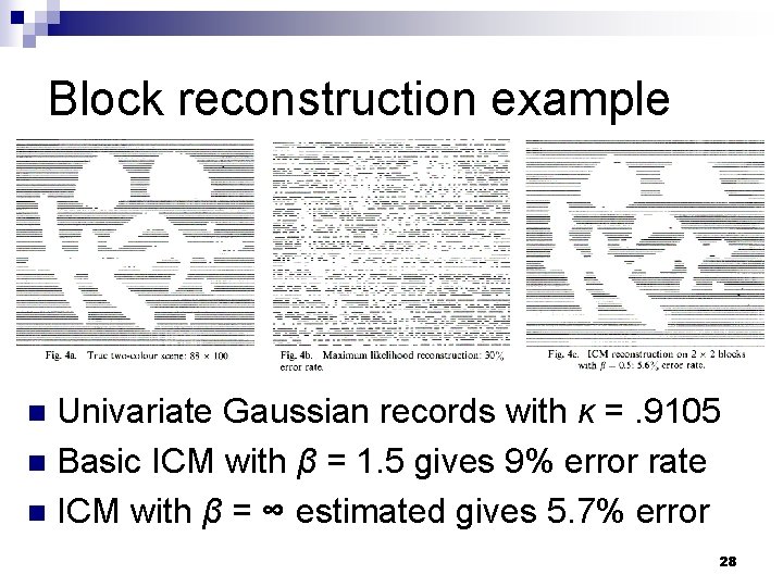
Block reconstruction example Univariate Gaussian records with κ =. 9105 n Basic ICM with β = 1. 5 gives 9% error rate n ICM with β = ∞ estimated gives 5. 7% error n 28

Conclusion n We began by adopting a strict probabilistic formulation with regard to the true scene and generated records. We then abandoned these in favor of ICM, on grounds of computation and to avoid unwelcome large-scale effects. There is a vast number of problems in image processing and pattern recognition to which statisticians might usefully contribute. 29