CHAPTER 10 Quantitative Data Analysis Quantitative Research Statistical

CHAPTER 10 Quantitative Data Analysis

Quantitative Research Statistical analysis is a tool and not an end to itself

HYPOTHESIS, ERRORS AND SIGNIFICANCE • You will have to develop a range of propositions, or suppositions that tentatively explains certain facts or phenomena. • The objective of the project is to provide information that you can then use to support the claim that your proposition is “true” or “false”. • The testing of hypotheses requires that you determine whether the results you have found did not occur by chance.

HYPOTHESIS • To statistically evaluate questions you need to put forward a hypothesis, which is an unproven testable proposition or supposition that tentatively explains certain facts or phenomena. • In its simplest form, the hypothesis is an “educated guess” based on the material that you have read.

HYPOTHESIS • The hypothesis is set up so that it will not be rejected (nullified) purely as a result of random error. • It is generally expressed in the negative i. e. there is no difference between “a” and “b”, or “a” and “b” are the same (i. e. a=b). • Rejecting this statement means that there is some difference between “a” and “b”, i. e. they are not equal.

Errors and Significance • When undertaking research you want to make sure that when you evaluate a hypothesis you: (a) do not randomly reject a null hypothesis that is true –Type 1 error OR (b) that you do not accept a null hypothesis that is false- Type II error. • The more certain you are that you have not committed a Type I error, the greater the chance is that you have committed Type II error!

Errors and Significance • What is the degree of error that I am willing to accept in my research? • Traditionally researchers say that they want to be 95% confident that the hypothesis is rejected, which is the same as a 5% chance of error or a probability level of 0. 05 that the hypothesis is in fact correct. • 95% (5%) of the observations will fall within (outside) a statistically determined range if the null hypothesis is true (False).

Errors and Significance • Select the hypothesis and the level of significance before undertaking the actual collection of data and empirical testing, as you need to ensure that you have the right kind of data and the level of “error” you are willing to accept. • An empirical test that is statistically significant means there is a difference, it does not identify the “importance” of a relationship. • It is possible to have large differences that are not significant or small differences that are.

EMPERICALLY EXAMINING DATA There are MANY ways to empirically look at data, included those that allow us to explore: • Basic analysis • Basic Associations • Comparing groups • Basic causal relationships • Advanced Techniques

10

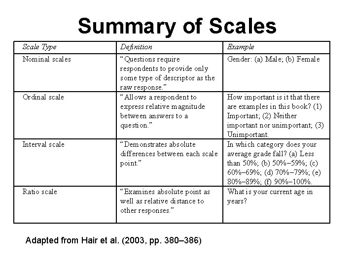
Summary of Scales Scale Type Definition Example Nominal scales “Questions require respondents to provide only some type of descriptor as the raw response. ” “Allows a respondent to express relative magnitude between answers to a question. ” Gender: (a) Male; (b) Female Ordinal scale Interval scale Ratio scale How important is it that there are examples in this book? (1) Important; (2) Neither important nor unimportant; (3) Unimportant. “Demonstrates absolute In which category does your differences between each scale average grade fall? (a) Less point. ” than 50%; (b) 50%– 59%; (c) 60%– 69%; (d) 70%– 79%; (e) 80%– 89%; (f) 90%– 100%. “Examines absolute point as What is your current age in well as relative distance to years? other responses. ” Adapted from Hair et al. (2003, pp. 380– 386)

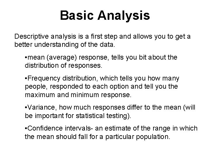
Basic Analysis Descriptive analysis is a first step and allows you to get a better understanding of the data. • mean (average) response, tells you bit about the distribution of responses. • Frequency distribution, which tells you how many people, responded to each option and tell you the maximum and minimum response. • Variance, how much responses differ to the mean (will be important for statistical testing). • Confidence intervals- an estimate of the range in which the mean should fall for a particular population.

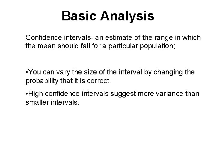
Basic Analysis Confidence intervals- an estimate of the range in which the mean should fall for a particular population; • You can vary the size of the interval by changing the probability that it is correct. • High confidence intervals suggest more variance than smaller intervals.

Sampling • You will not be able to collect data from everyone in your population of interest, thus you will have a sample that is representative of this group. • There may be many factors that affect your sample, demographics, when you collect the data, etc.

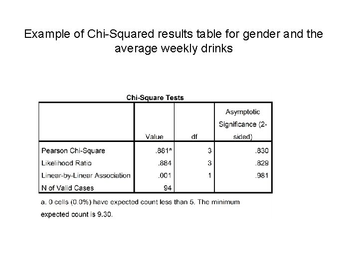
Cross Tabulations You examine responses across two or more variables at the same time. • Chi-squared is basis test as to whether the respondents are distributed as expected based on the two variables. • This is a kind of test of association, but again does not tell us A causes B, only that A and B are related.

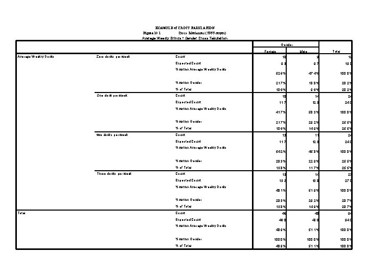
EXAMPLE of CROSS TABULATION Figure 10. 1 Cross-Tabulations (SPSS output) Average Weekly Drinks * Gender Cross Tabulation Gender Female Average Weekly Drinks Zero drinks per week 10 9 19 Expected Count 9. 3 9. 7 19. 0 52. 6% 47. 4% 100. 0% % within Gender 21. 7% 18. 8% 20. 2% % of Total 10. 6% 9. 6% 20. 2% 10 14 24 11. 7 12. 3 24. 0 41. 7% 58. 3% 100. 0% % within Gender 21. 7% 29. 2% 25. 5% % of Total 10. 6% 14. 9% 25. 5% 13 11 24 11. 7 12. 3 24. 0 54. 2% 45. 8% 100. 0% % within Gender 28. 3% 22. 9% 25. 5% % of Total 13. 8% 11. 7% 25. 5% 13 14 27 13. 2 13. 8 27. 0 48. 1% 51. 9% 100. 0% % within Gender 28. 3% 29. 2% 28. 7% % of Total 13. 8% 14. 9% 28. 7% % within Average Weekly Drinks One drink per week Count Expected Count % within Average Weekly Drinks two drinks per week Count Expected Count % within Average Weekly Drinks Three drinks per week Count Expected Count % within Average Weekly Drinks Total Male Count Expected Count % within Average Weekly Drinks % within Gender % of Total 46 48 94 46. 0 48. 0 94. 0 48. 9% 51. 1% 100. 0% 48. 9% 51. 1% 100. 0%

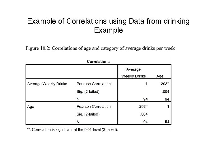
Basic Associations • Correlations tell you the extent to which that two variables move together ranging from +1 to – 1. • There are different types that can be used on different types of data. • The closer to 1 (positive or negative) the more directly the two items move together. • We also need to consider the significance, i. e. is the relationship random. • WE DO NOT however know that one causes the other!

Example of Correlations using Data from drinking Example

Example of Chi-Squared results table for gender and the average weekly drinks

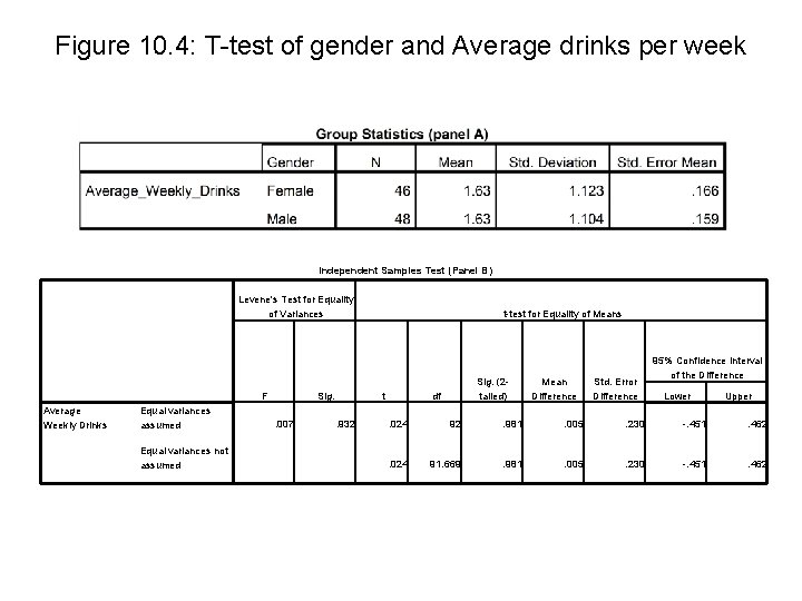
Comparing Groups • Z-test – compares portions between 2 groups. For example do the same portions of students get HD based on whether they are face-to-face or off-campus? • t-test, which compares the mean values between 2 groups. • With both there is a p-value indicating whether the difference is statically different.

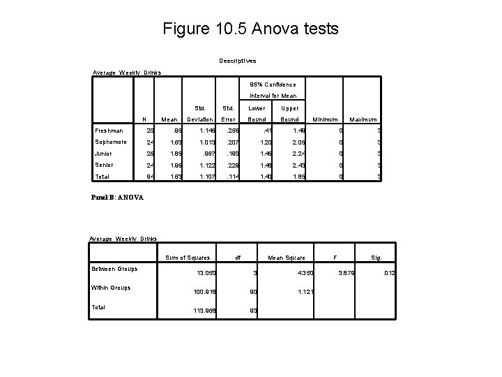
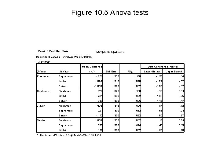
Comparing Groups • Analysis of variance (Anova) do means of one variable (or interacting variables) differ across multiple groups. This does not tell you which group or groups differ. • Multiple Analysis of Variance (MANOVA)- technique has the benefit of identifying whether a set of variables differs between two groups, thus you do not have the multiple comparison problem identified earlier.

Figure 10. 4: T-test of gender and Average drinks per week Independent Samples Test (Panel B) Levene's Test for Equality of Variances F Average Weekly Drinks Equal variances assumed Equal variances not assumed Sig. . 007 t-test for Equality of Means t. 932 Sig. (2 tailed) df Mean Difference Std. Error Difference 95% Confidence Interval of the Difference Lower Upper . 024 92 . 981 . 005 . 230 -. 451 . 462 . 024 91. 669 . 981 . 005 . 230 -. 451 . 462

Figure 10. 5 Anova tests Descriptives Average_Weekly_Drinks 95% Confidence Interval for Mean N Mean Std. Lower Upper Deviation Error Bound Minimum Maximum Freshman 20 . 95 1. 146 . 256 . 41 1. 49 0 3 Sophomore 24 1. 63 1. 013 . 207 1. 20 2. 05 0 3 Junior 26 1. 85 . 967 . 190 1. 46 2. 24 0 3 Senior 24 1. 96 1. 122 . 229 1. 48 2. 43 0 3 Total 94 1. 63 1. 107 . 114 1. 40 1. 85 0 3 Panel B: ANOVA Average_Weekly_Drinks Sum of Squares Between Groups Within Groups Total df Mean Square F Sig. 3. 879 . 012 13. 050 3 4. 350 100. 918 90 1. 121 113. 968 93

Figure 10. 5 Anova tests Panel C Post Hoc Tests Multiple Comparisons Dependent Variable: Average Weekly Drinks Tukey HSD Mean Difference (I) Year (J) Year Freshman Sophomore -. 675 . 321 . 159 -1. 51 . 16 Junior -. 896* . 315 . 028 -1. 72 -. 07 Senior -1. 008* . 321 . 012 -1. 85 -. 17 . 675 . 321 . 159 -. 16 1. 51 Junior -. 221 . 300 . 882 -1. 01 . 56 Senior -. 333 . 306 . 696 -1. 13 . 47 Freshman . 896* . 315 . 028 . 07 1. 72 Sophomore . 221 . 300 . 882 -. 56 1. 01 -. 112 . 300 . 982 -. 90 . 67 1. 008* . 321 . 012 . 17 1. 85 Sophomore . 333 . 306 . 696 -. 47 1. 13 Junior . 112 . 300 . 982 -. 67 . 90 Sophmore Junior Freshman Senior Freshman (I-J) 95% Confidence Interval Std. Error *. The mean difference is significant at the 0. 05 level. Sig. Lower Bound Upper Bound

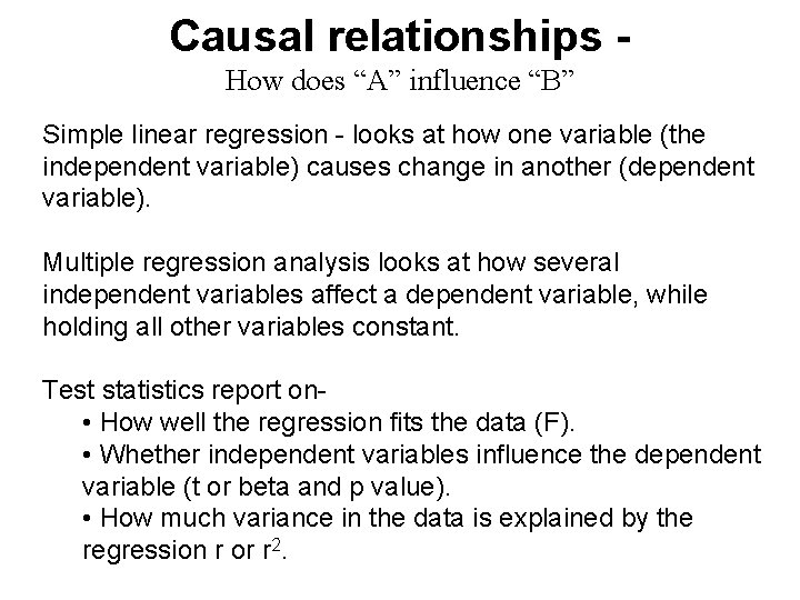
Causal relationships How does “A” influence “B” Simple linear regression - looks at how one variable (the independent variable) causes change in another (dependent variable). Multiple regression analysis looks at how several independent variables affect a dependent variable, while holding all other variables constant. Test statistics report on- • How well the regression fits the data (F). • Whether independent variables influence the dependent variable (t or beta and p value). • How much variance in the data is explained by the regression r or r 2.

Advanced Techniques • Factor analysis - groups variables that move in similar ways, which are often added together (aggregated) into one variable (called a composite construct). • Cluster analysis - groups individuals based on their responses to questions. It is used in segmentation studies that differentiate groups based on how they respond to questions, rather than on simple demographic variables. The groups can then be used in other analysis. • Structurally equation modelling allows you to identify how variables relate within complex systems of relationships, moving beyond multiple regression.

Advanced Techniques Conjoint analysis or Choice modelling allows the researcher to provide respondents with different alternatives, where attributes are varied and the researcher can empirically determine the value of each attribute to the individual.

Conclusions • The analysis technique will directly relate to your research question. • Thus you need to know what you want to explore when designing your topic and then ensure you collect the right kind of data. • In many cases you will possibly use multiple methods to assist with aspects of the research issue. • In thinking about what you need to learn about, you will need to include, learning how to undertake your analysis!

Project Checklist • Will your project have a quantitative component? • Have you collected the right data for the analysis you want to do? • Who will be in charge of this? • When will it occur? • What preparation must be done? • Who will interpret the data, and how will it be interpreted?