The Geometry of Virtual Worlds CS 498 VR

The Geometry of Virtual Worlds CS 498 VR: Virtual Reality UNIVERSITY OF ILLINOIS AT URBANA-CHAMPAIGN Eric Shaffer

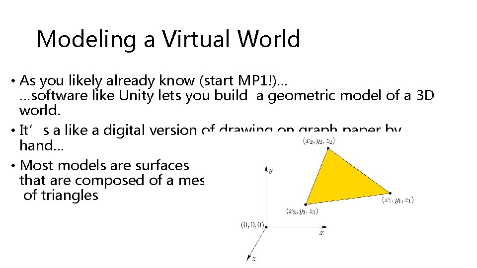
Modeling a Virtual World • As you likely already know (start MP 1!)… …software like Unity lets you build a geometric model of a 3 D world. • It’s a like a digital version of drawing on graph paper by hand… • Most models are surfaces that are composed of a mesh of triangles

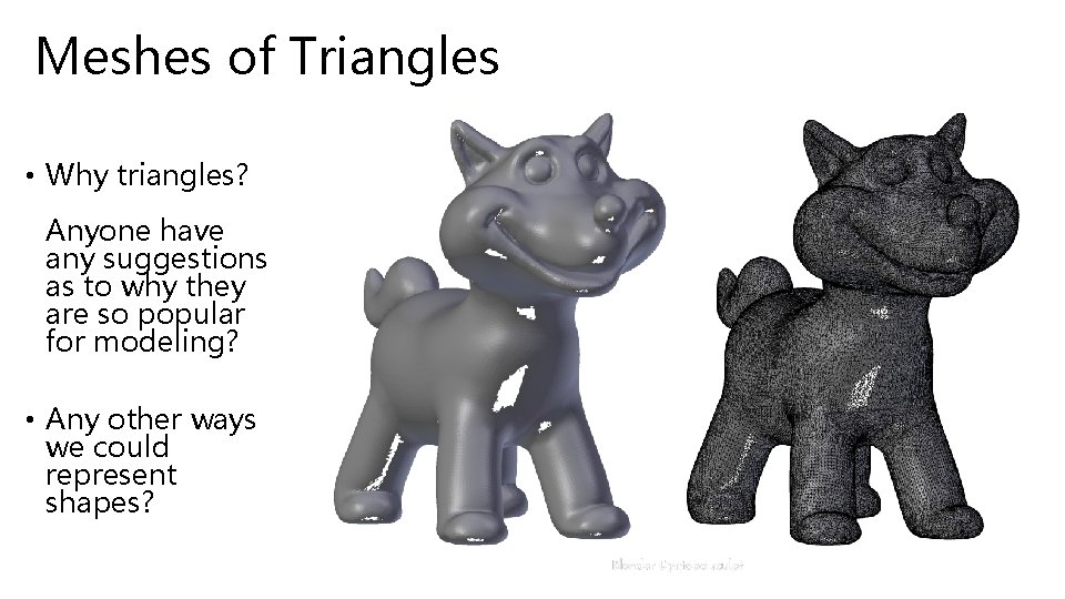
Meshes of Triangles • Why triangles? Anyone have any suggestions as to why they are so popular for modeling? • Any other ways we could represent shapes?

Geometric Modeling Fundamentals… • We will discuss basic geometric modeling for 3 D computer graphics • As the book says…. If you work with high-level engines to build a VR experience, then most of the concepts from this chapter might not seem necessary. You might need only to select options from menus and write simple scripts. However, an understanding of the basic transformations, such as how to express 3 D rotations or move a camera viewpoint, is essential to making the software do what you want. - S. M. Lavalle, Virtual Reality It’s easier to use tools when you know how they work.

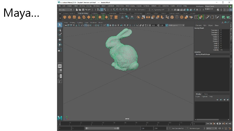
How DO You Generate a Mesh? • Often generated using a modeling tool like Maya or Blender • Both freely available • Export your model as file…. . • Import it into Unity…. .

Maya…

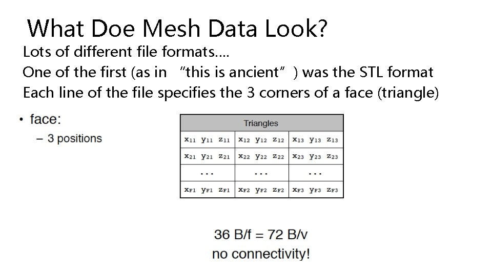
What Doe Mesh Data Look? Lots of different file formats…. One of the first (as in “this is ancient”) was the STL format Each line of the file specifies the 3 corners of a face (triangle)

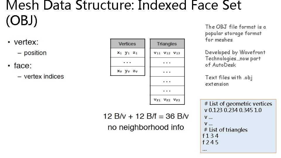
Mesh Data Structure: Indexed Face Set (OBJ) The OBJ file format is a popular storage format for meshes Developed by Wavefront Technologies…now part of Auto. Desk Text files with. obj extension # List of geometric vertices v 0. 123 0. 234 0. 345 1. 0 v. . . # List of triangles f 134 f 245 …

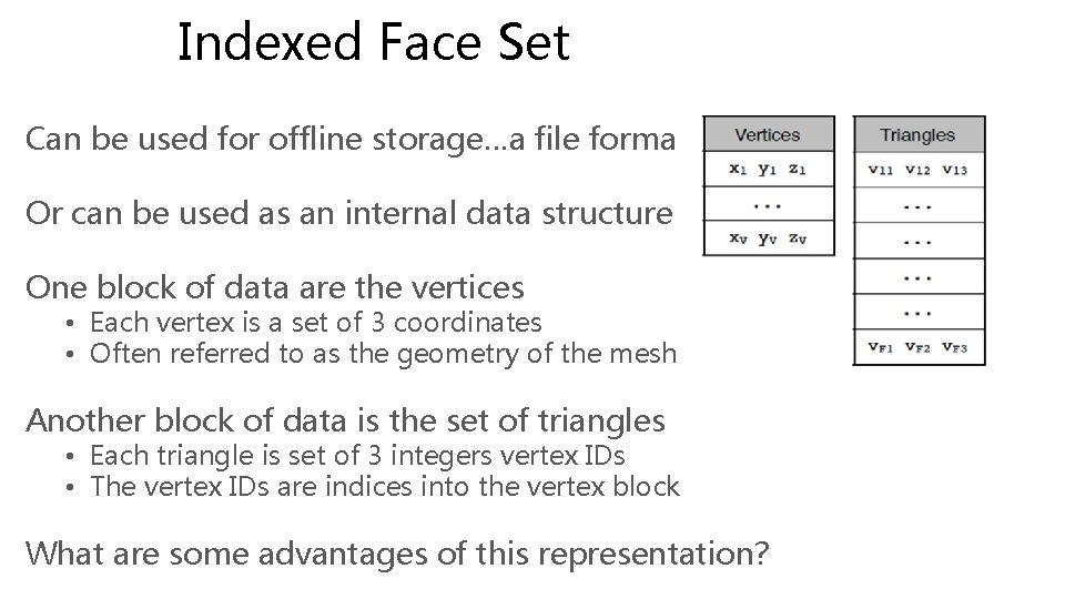
Indexed Face Set Can be used for offline storage…a file format Or can be used as an internal data structure One block of data are the vertices • Each vertex is a set of 3 coordinates • Often referred to as the geometry of the mesh Another block of data is the set of triangles • Each triangle is set of 3 integers vertex IDs • The vertex IDs are indices into the vertex block What are some advantages of this representation?

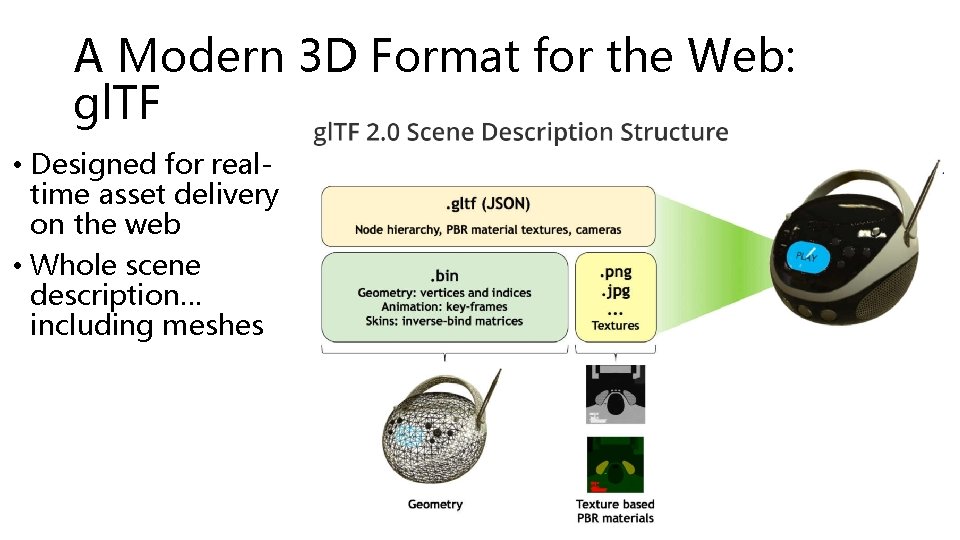
A Modern 3 D Format for the Web: gl. TF • Designed for realtime asset delivery on the web • Whole scene description… including meshes

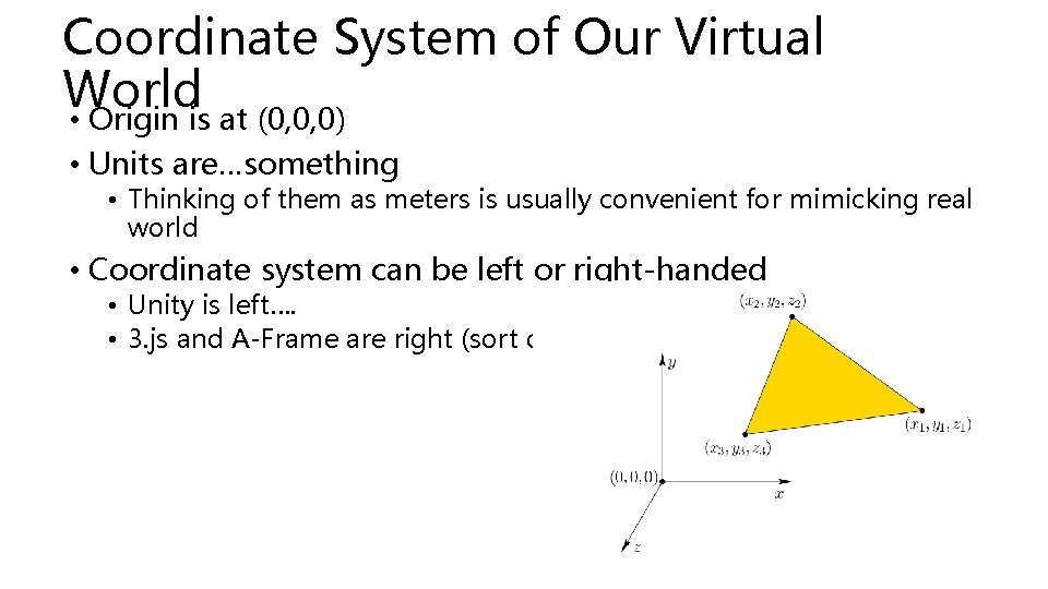
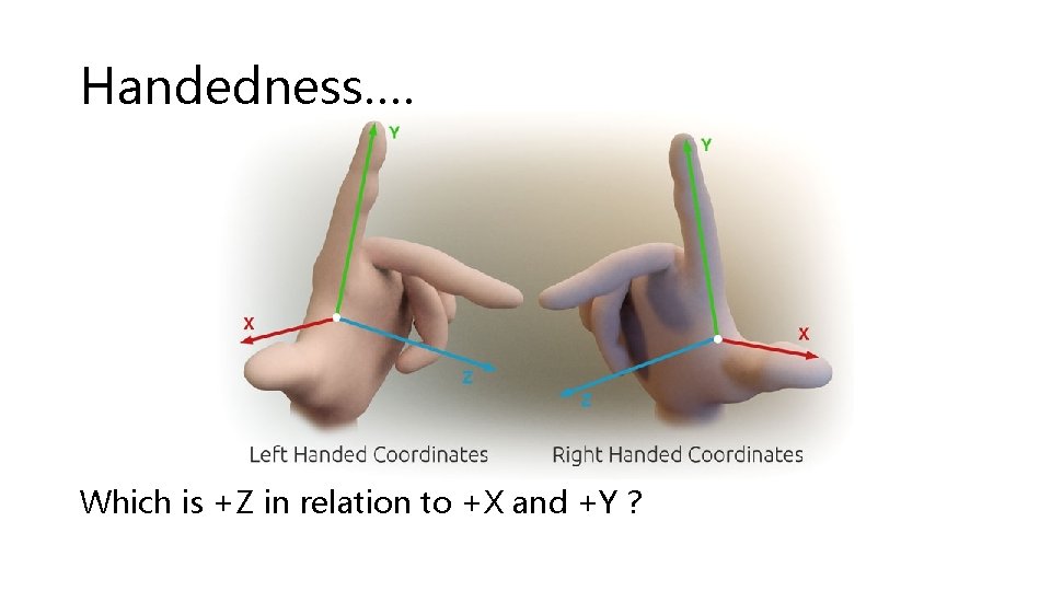
Coordinate System of Our Virtual World • Origin is at (0, 0, 0) • Units are…something • Thinking of them as meters is usually convenient for mimicking real world • Coordinate system can be left or right-handed • Unity is left…. • 3. js and A-Frame are right (sort of)…

Handedness…. Which is +Z in relation to +X and +Y ?

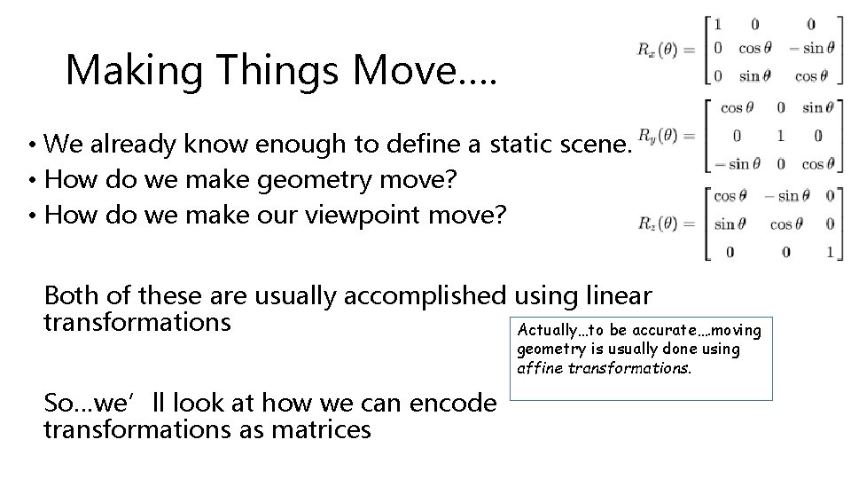
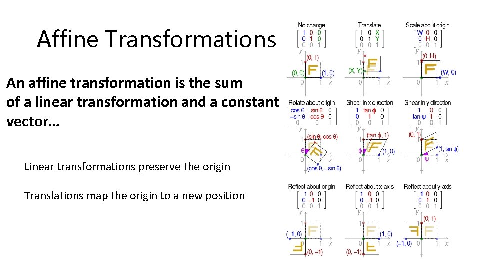
Making Things Move…. • We already know enough to define a static scene… • How do we make geometry move? • How do we make our viewpoint move? Both of these are usually accomplished using linear transformations Actually…to be accurate…. moving geometry is usually done using affine transformations. So…we’ll look at how we can encode transformations as matrices

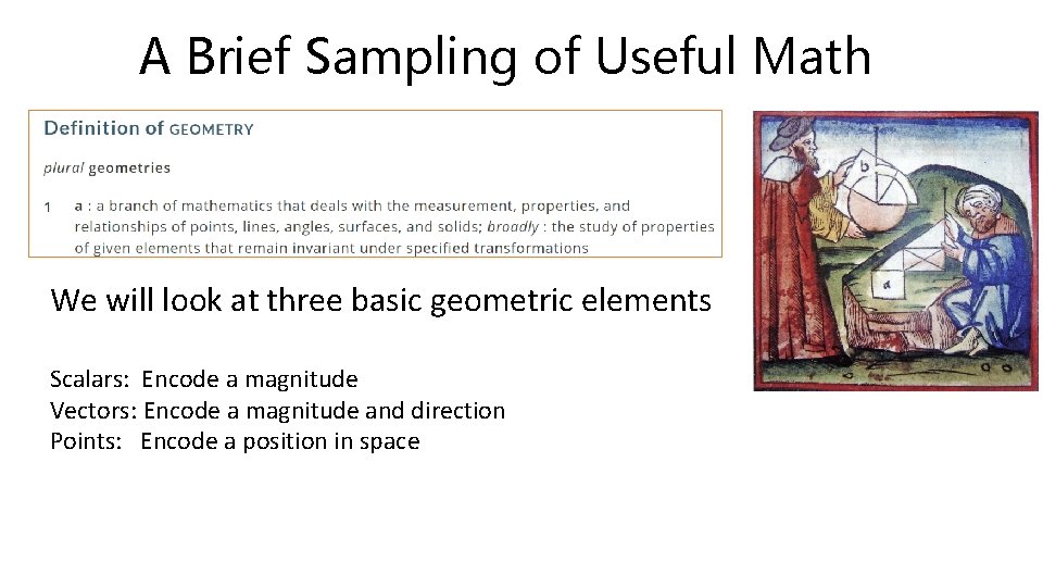
A Brief Sampling of Useful Math We will look at three basic geometric elements Scalars: Encode a magnitude Vectors: Encode a magnitude and direction Points: Encode a position in space

Scalars are quantities which express only a magnitude… Think of them as just a single number like 3. 14 Scalars: • members of a set which • can be combined by two operations (addition and multiplication) • obey some fundamental laws (associativity, commutativity, inverses) Examples include the real numbers • under the ordinary arithmetic rules with which we are familiar

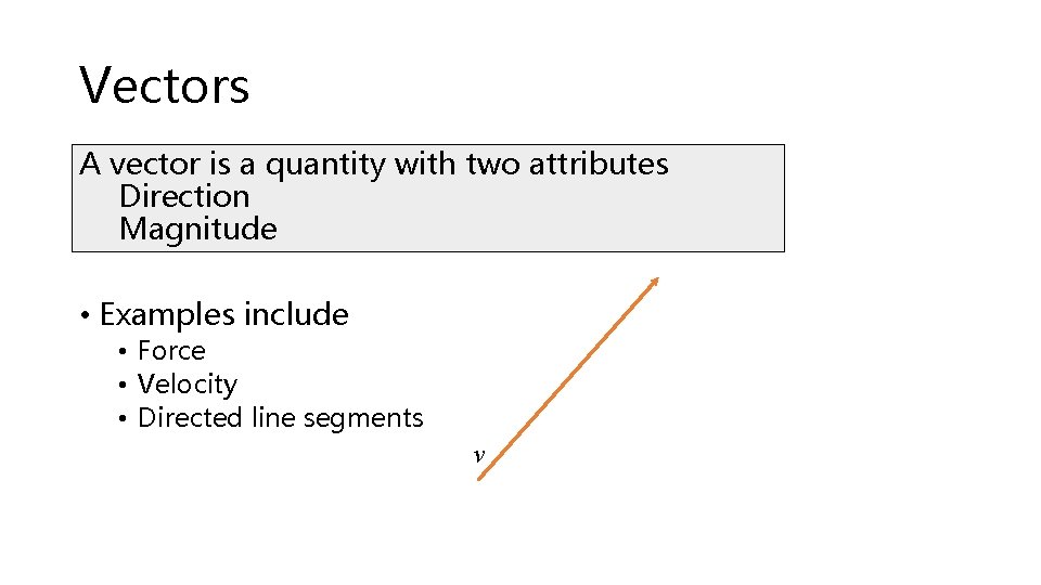
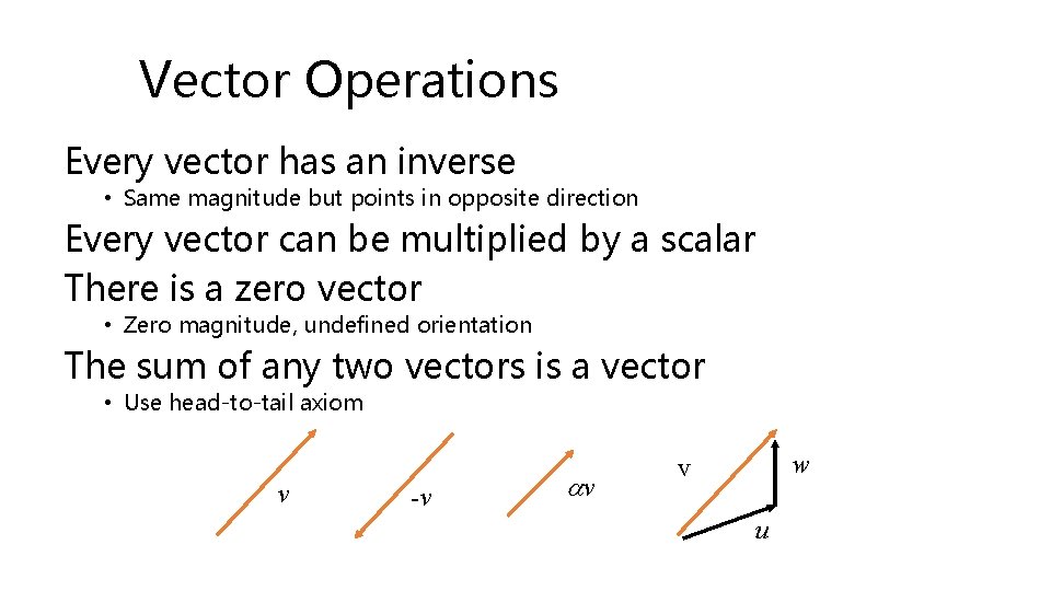
Vectors A vector is a quantity with two attributes Direction Magnitude • Examples include • Force • Velocity • Directed line segments v

Vector Operations Every vector has an inverse • Same magnitude but points in opposite direction Every vector can be multiplied by a scalar There is a zero vector • Zero magnitude, undefined orientation The sum of any two vectors is a vector • Use head-to-tail axiom v -v v w v u

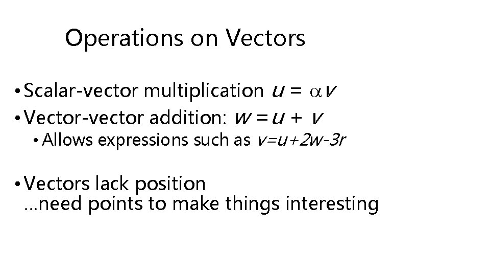
Operations on Vectors • Scalar-vector multiplication u = v • Vector-vector addition: w =u + v • Allows expressions such as v=u+2 w-3 r • Vectors lack position …need points to make things interesting

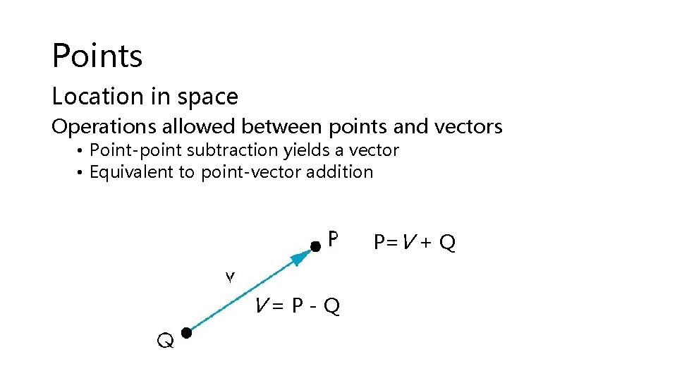
Points Location in space Operations allowed between points and vectors • Point-point subtraction yields a vector • Equivalent to point-vector addition P=V + Q V=P-Q

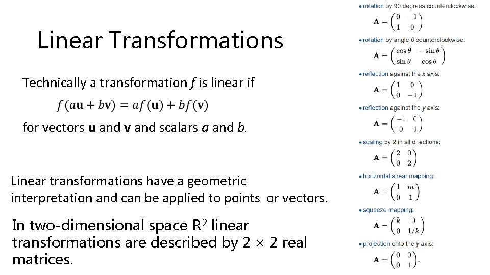
Linear Transformations Technically a transformation f is linear if for vectors u and v and scalars a and b. Linear transformations have a geometric interpretation and can be applied to points or vectors. In two-dimensional space R 2 linear transformations are described by 2 × 2 real matrices.

Affine Transformations An affine transformation is the sum of a linear transformation and a constant vector… Linear transformations preserve the origin Translations map the origin to a new position

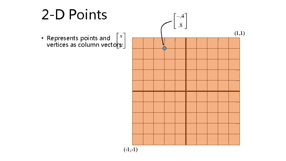
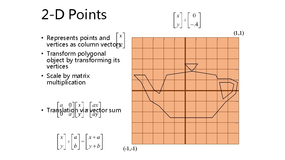
2 -D Points (1, 1) • Represents points and vertices as column vectors: (-1, -1)

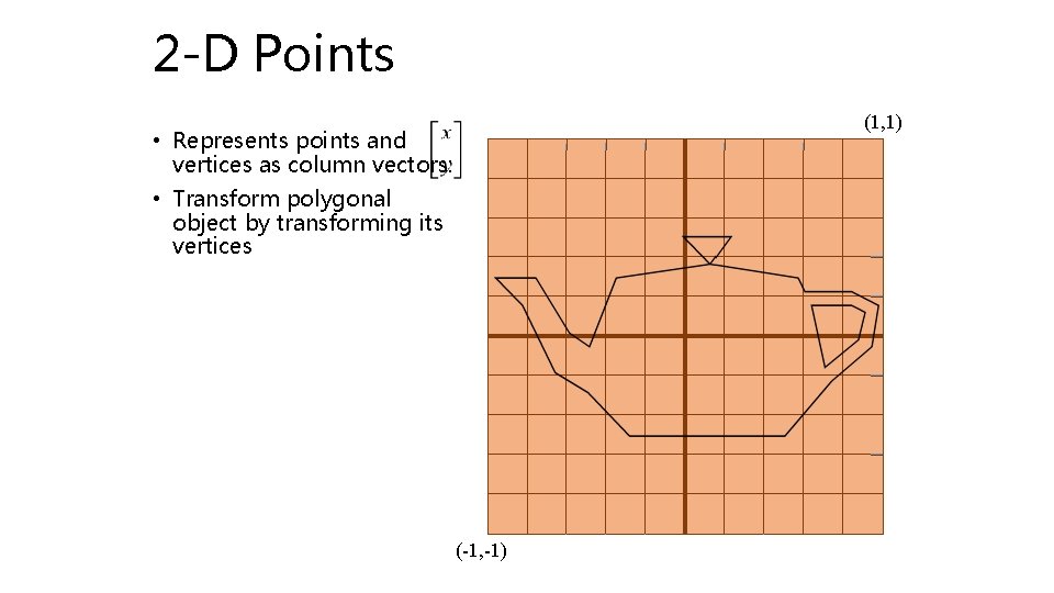
2 -D Points (1, 1) • Represents points and vertices as column vectors: • Transform polygonal object by transforming its vertices (-1, -1)

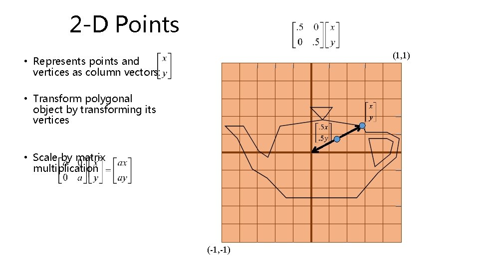
2 -D Points (1, 1) • Represents points and vertices as column vectors: • Transform polygonal object by transforming its vertices • Scale by matrix multiplication (-1, -1)

2 -D Points (1, 1) • Represents points and vertices as column vectors: • Transform polygonal object by transforming its vertices • Scale by matrix multiplication • Translation via vector sum (-1, -1)

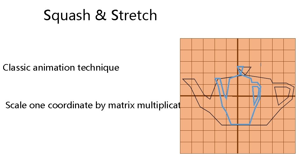
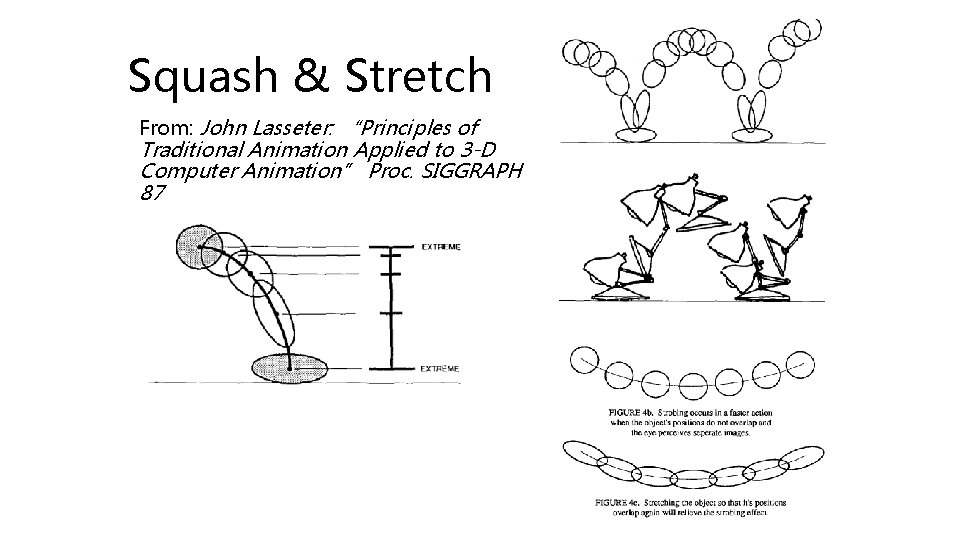
Squash & Stretch Classic animation technique Scale one coordinate by matrix multiplication

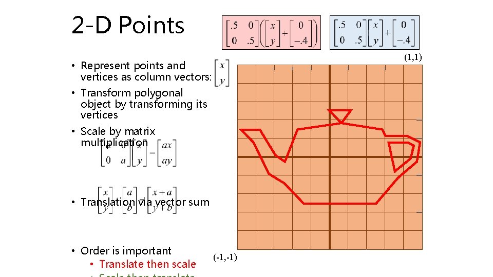
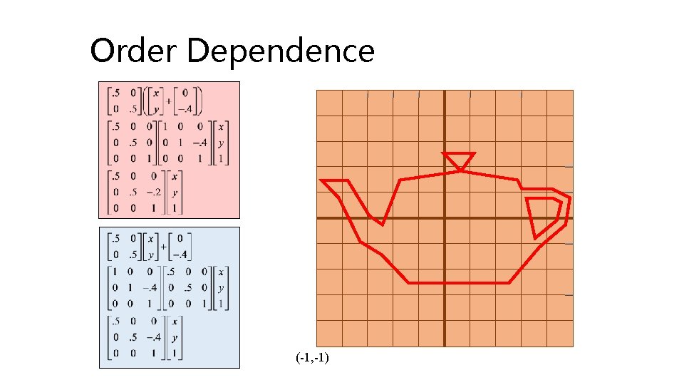
2 -D Points (1, 1) • Represent points and vertices as column vectors: • Transform polygonal object by transforming its vertices • Scale by matrix multiplication • Translation via vector sum • Order is important • Translate then scale (-1, -1)

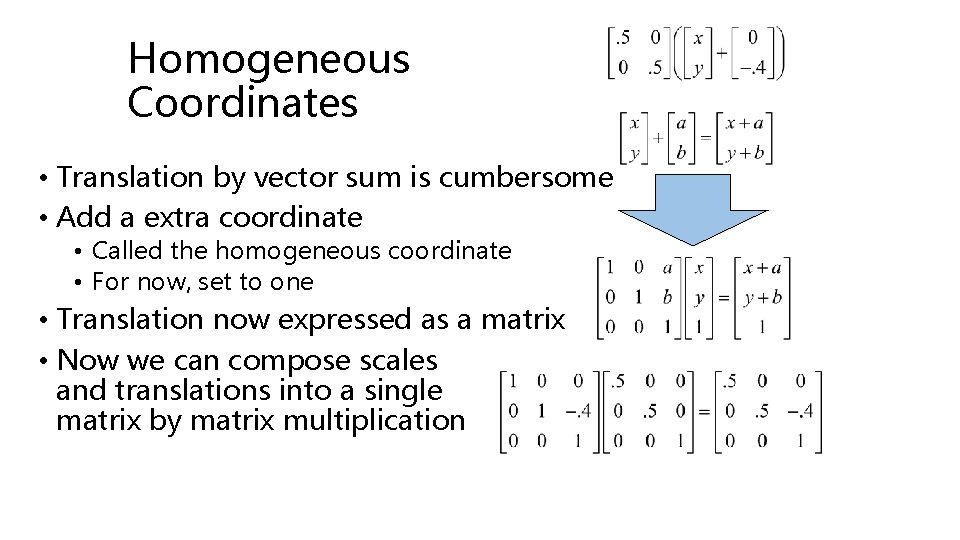
Homogeneous Coordinates • Translation by vector sum is cumbersome • Add a extra coordinate • Called the homogeneous coordinate • For now, set to one • Translation now expressed as a matrix • Now we can compose scales and translations into a single matrix by matrix multiplication

Order Dependence (-1, -1)

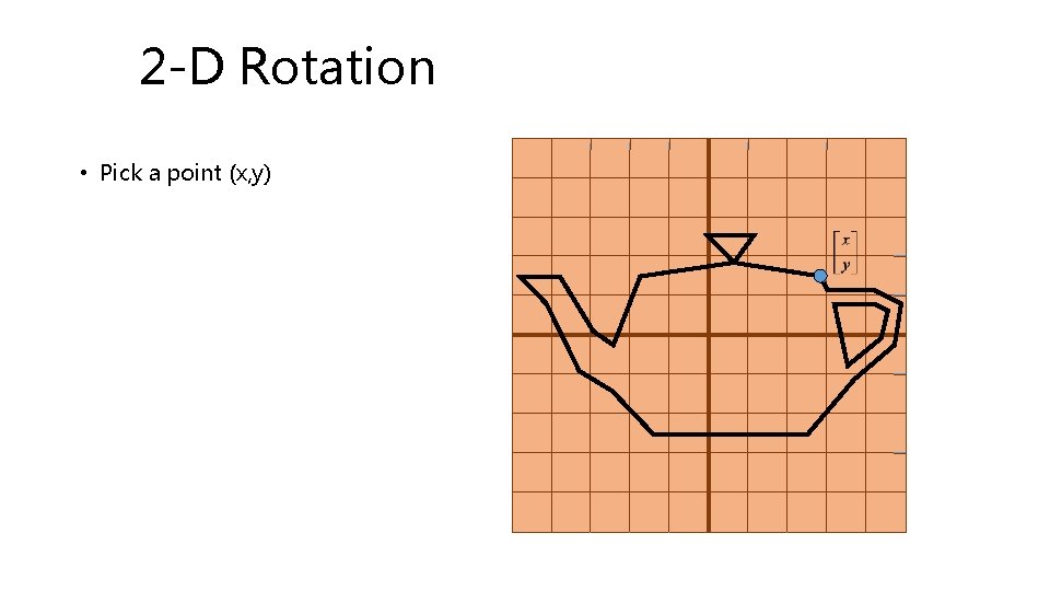
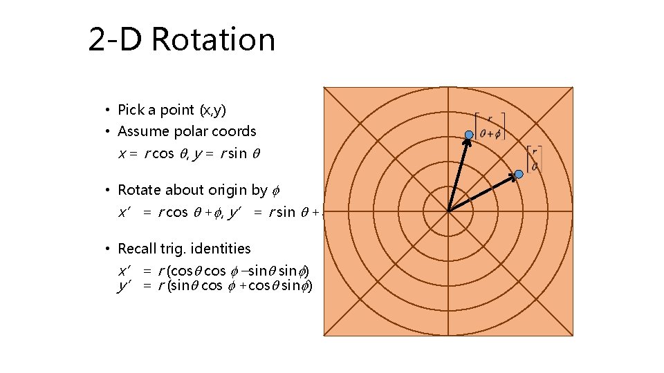
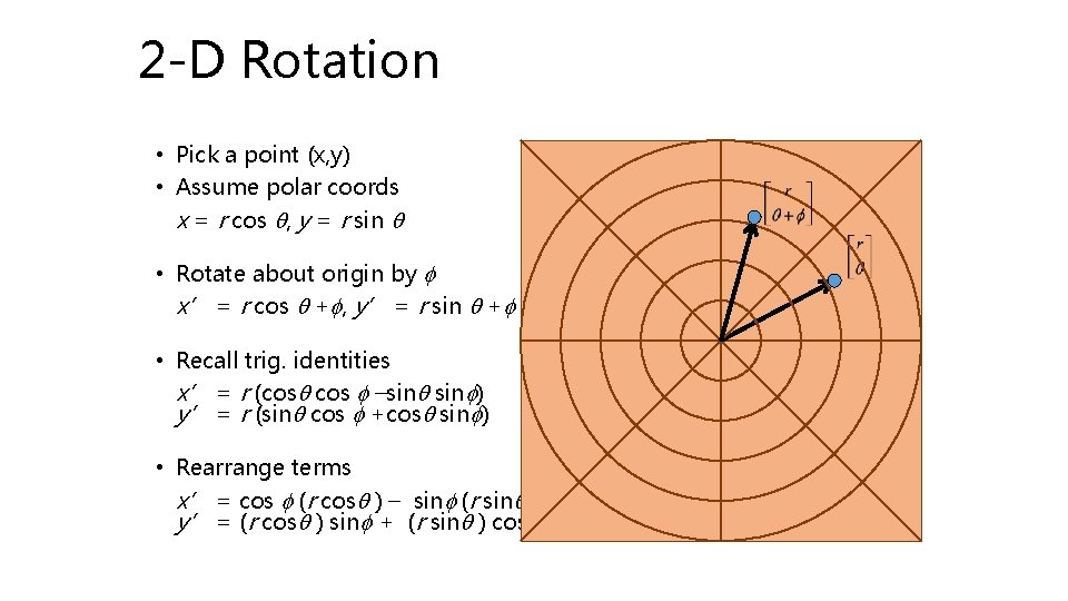
2 -D Rotation • Pick a point (x, y)

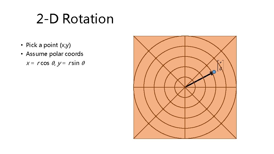
2 -D Rotation • Pick a point (x, y) • Assume polar coords x = r cos q, y = r sin q

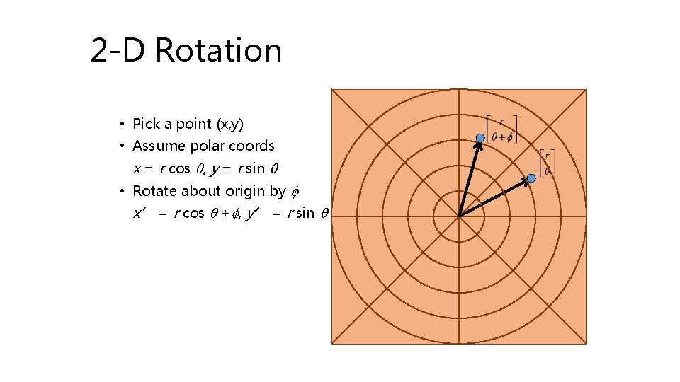
2 -D Rotation • Pick a point (x, y) • Assume polar coords x = r cos q, y = r sin q • Rotate about origin by f x’ = r cos q +f, y’ = r sin q +f

2 -D Rotation • Pick a point (x, y) • Assume polar coords x = r cos q, y = r sin q • Rotate about origin by f x’ = r cos q +f, y’ = r sin q +f • Recall trig. identities x’ = r (cosq cos f –sinq sinf) y’ = r (sinq cos f +cosq sinf)

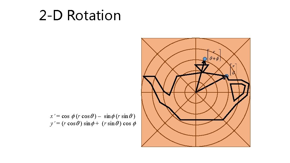
2 -D Rotation • Pick a point (x, y) • Assume polar coords x = r cos q, y = r sin q • Rotate about origin by f x’ = r cos q +f, y’ = r sin q +f • Recall trig. identities x’ = r (cosq cos f –sinq sinf) y’ = r (sinq cos f +cosq sinf) • Rearrange terms x’ = cos f (r cosq ) – sinf (r sinq ) y’ = (r cosq ) sinf + (r sinq ) cos f

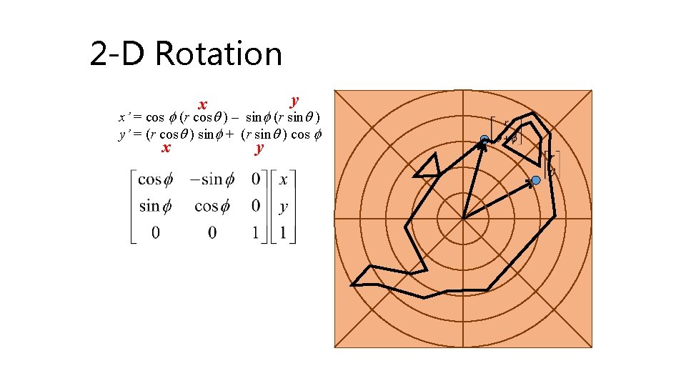
2 -D Rotation x’ = cos f (r cosq ) – sinf (r sinq ) y’ = (r cosq ) sinf + (r sinq ) cos f

2 -D Rotation y x x’ = cos f (r cosq ) – sinf (r sinq ) y’ = (r cosq ) sinf + (r sinq ) cos f x y

Squash & Stretch From: John Lasseter: “Principles of Traditional Animation Applied to 3 -D Computer Animation” Proc. SIGGRAPH 87

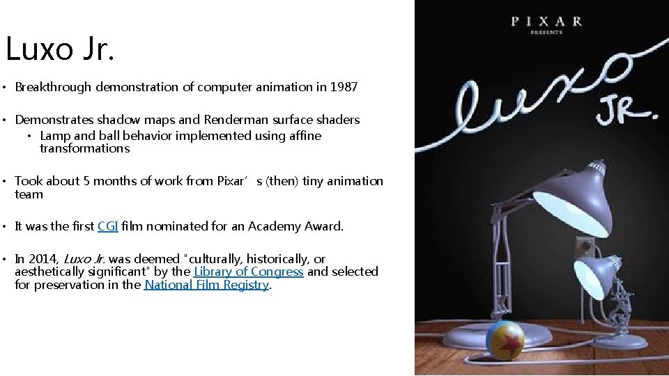
Luxo Jr. Directed by John Lasseter Written by John Lasseter Production company Pixar Release date Aug. 17, 1986 (SIGGRAPH)

Luxo Jr. • Breakthrough demonstration of computer animation in 1987 • Demonstrates shadow maps and Renderman surface shaders • Lamp and ball behavior implemented using affine transformations • Took about 5 months of work from Pixar’s (then) tiny animation team • It was the first CGI film nominated for an Academy Award. • In 2014, Luxo Jr. was deemed "culturally, historically, or aesthetically significant" by the Library of Congress and selected for preservation in the National Film Registry.

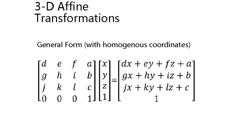
3 -D Affine Transformations General Form (with homogenous coordinates)

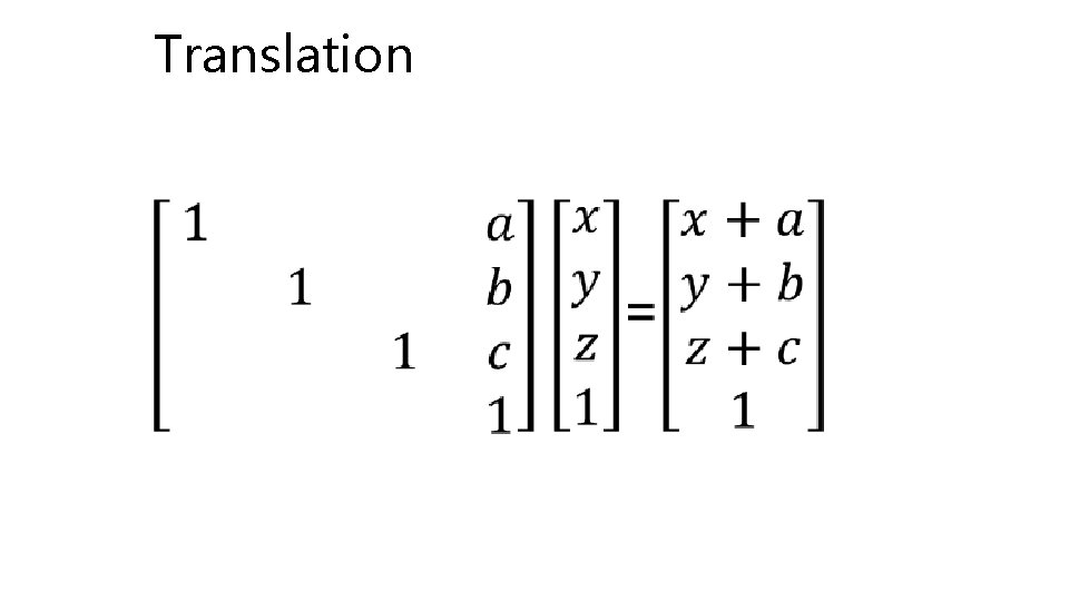
Translation

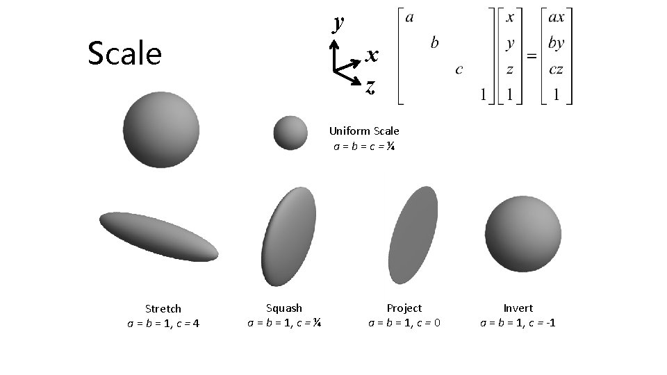
y Scale x z Uniform Scale a=b=c=¼ Stretch a = b = 1, c = 4 Squash a = b = 1, c = ¼ Project a = b = 1, c = 0 Invert a = b = 1, c = -1

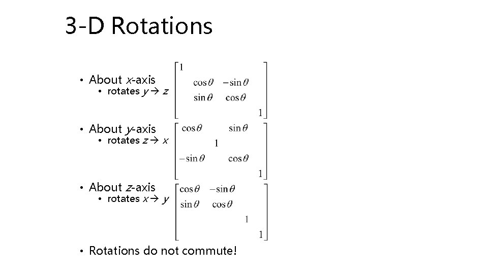
3 -D Rotations • About x-axis • rotates y z • About y-axis • rotates z x • About z-axis • rotates x y • Rotations do not commute!

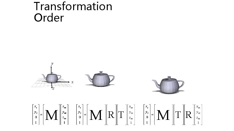
Transformation Order y x z M M RT M T R