Imaging Geometry 1 Imaging Geometry o Imaging Geometry

Imaging Geometry: 1

Imaging Geometry: o Imaging Geometry plays a very important part in Image processing, as it deals with the techniques and transformation for mapping Real world objects and their characteristics on Image plane. o Any point in 3 D co ordinate system is represented by BLOCK letters, termed as World Coordinate system. n o W(X, Y, Z) Any point in 2 D co ordinate system / Image plane is represented by small letters, termed as Camera coordinate system. n f (x, y) 2

Translation: Y P 2(X 2, Y 2, Z 2) (dx, dy, dz) P 1(X 1, Y 1, Z 1) X Z 3

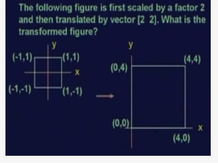
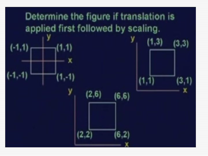
Translation: o o Suppose that the task is to translate a point P 1, with coordinate values (x 1 , y 1 , z 1 ) to new location P 2, by Using displacement ( dx , dy , dz). The translation is easily accomplished by using the equation: X 2 = X 1 + dx Y 2 = Y 1 + dy Z 2 = Z 1 + dz ===>(i) ===>(iii) 4

Translation: o o Where (X 2, Y 2, Z 2) are new points and can be represented in Matrix form, as: X 2 y 2 z 2 V* = 100 010 001 T dx dy dz x 1 y 1 z 1 V where, V* is the new point, T is the translation matrix, and V is the original point. 5

Translation: o Here, the product of Matrices T & V seems Invalid, As Columns of T = Rows of V o So we can generalize this transformation by inserting a DUMMY row in all three matrices. V* = T X 2 100 y 2 010 z 2 001 1 000 T = 1 0 0 0 0 1 0 dx dy dz 1 V x 1 y 1 z 1 1 Translation Matrix 6

Inverse Translation: o The Initial Point P 1 can be traced back by applying the Inverse Translation, that is: V = X 1 y 1 z 1 1 T-1 = T-1 V* 1 0 0 0 0 1 0 -dx -dy -dz 1 x 2 y 2 z 2 1 Inverse Translation Matrix I 7

Translation: Original Image translated at 200 pixels from top and 100 pixels from left MUET Central Library 8

Translation: Image translated at 300 pixels from top and 200 pixels from left Image translated at 500 pixels from top and 300 pixels from left MUET Central Library 9

Translation: Image translated at 350 pixels from bottom and 200 pixels from right Image translated at 400 pixels from bottom and 300 pixels from right MUET Central Library 10

Translation: Image translated at 500 pixels from bottom and 300 pixels from right Image translated at 500 pixels from top and 300 pixels from left This property is used in adjusting the Objects on Monitor screen. MUET Central Library 11

Scaling: o The scale operator performs a geometric transformation which can be used to shrink or zoom the size of an image. o The shrink or Zoom, depends upon the vales of scaling factor. o For values between 0 &1, the resultant Image is shrinked. o For values greater than 1, the resultant Image is expanded by that factor. 12

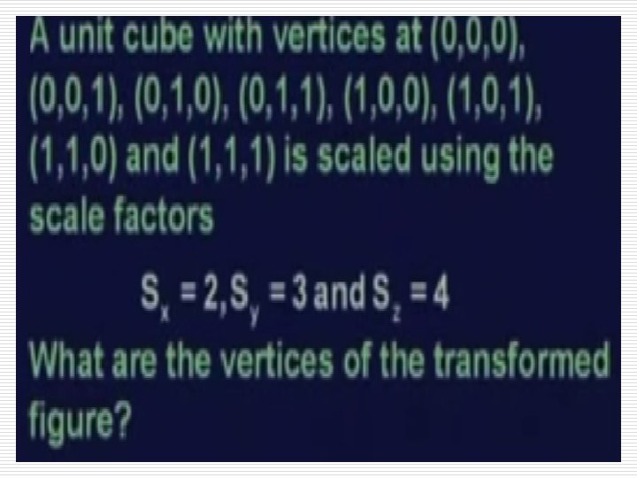
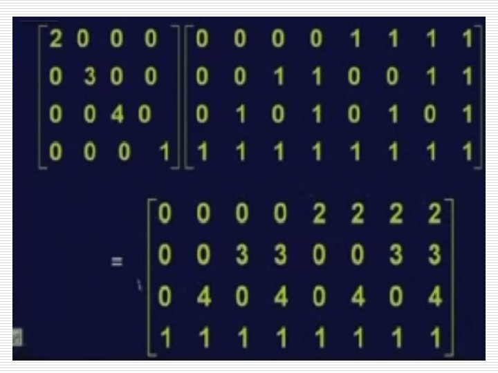
Scaling: o o The Scaling is easily accomplished by using the equations: X 2 = X 1 * sx ===>(i) Y 2 = Y 1 * sy Z 2 = Z 1 * sz ===>(ii) ===>(iii) Where (X 2, Y 2, Z 2) are new points and expressed in Matrix form as: V* = T X 2 Y 2 Z 2 1 sx = 0 0 sy 0 0 V 0 0 sz 0 0 1 X 1 Y 1 Z 1 1 Where T represents the Scaling Matrix. 13

Scaling: Original Image shrinked at scaling factor of. 5 MUET Central Library 14

Scaling: o The Initial Scale can be traced back by applying the Inverse Scaling, that is: V X 1 y 1 z 1 1 T-1 T. T-1 = = T-1 1/Sx 0 0 0 V* 0 1/Sy 0 0 1/Sz 1/Sx 0 0 1/Sy 0 0 0 1/Sz 0 0 1 x 2 y 2 z 2 1 0 0 0 1 Inverse Scaling Matrix I 15

Rotation : o The transformation used for 3 -D rotation is inherently more complex than the Transformations discussed so far. o The simplest form of these transformations is for Rotation of a point about the coordinate axes. o To rotate a point about another arbitrary Point in space, we require three transformation: n n n The first translate the arbitrary point to the Origin, The second performs the rotation, and The third translates the point back to its Original position. 16

Rotation : o Rotation of a point about the Z coordinate axis by an angle is achieved by using the transformation. o The rotation angle is measured clockwise when looking at the region from a Point on the +Z axis. This transformation affects only the values of X and Y coordinates. o The rotation operator performs a geometric transform which maps the position ( x 1, y 1 ) of a picture element in an input image onto a position ( x 2, y 2 ) in an output image by rotating it through a user-specified angle ө about an origin (0, 0). 17

Rotation along Z-axis: Y P 2(X 2, Y 2, Z 2) R is length of vector. R Y 1 Y 2 φ is initial angle with X axis. P 1(X 1, Y 1, Z 1) R θ 0 φ X X 2 X 1 Z 18

Rotation along Z-axis: o Assume that the Vector (R) is making an angle of φ with X axis. o So initially, the components can be achieved as: n n n o X 1=R cos φ Y 1=R sin φ Z 1=Z 1 If we rotate the vector R by θ around Z-axis in Counter clock wise Direction, then new point formed will be given by: n n n X 2=R cos (φ+θ) Y 2=R sin (φ+θ ) Z 2=Z 1 (Un changed axis) 19

Rotation along Z-axis: o By expanding the terms of Sin and Cosine, we get: X 2 = Y 2 = Z 2= o R cosθ cosφ R sinθ cosφ Z 1 R sinφ sinθ R sinφ cosθ But, we have assumed initially that: R cosφ=x 1 R sinφ=y 1 o + ===>(a) ===>(b) So our new point (x 2, Y 2, z 2) becomes: X 2 = Y 2 = z 2= X 1 cosθ X 1 sinθ z 1 - Y 1 sinθ + Y 1 cosθ 20

Rotation along Z-axis: o For matrix representation, these equations can be interpreted as: X 2 = X 1 cosθ Y 2 = X 1 sinθ z 2 = 0 o - Y 1 sinθ + Y 1 cosθ + 0 + + 0 0 + z 1 In form of matrices, the rotation operation can be given as: x 2 y 2 z 2 cosθ sinθ 0 -sinθ cosθ 0 V* = Rθ Z 0 0 1 x 1 y 1 z 1 V 21

Inverse Rotation along Z-axis: In form of matrices, the Inverse rotation operation can be given as: V x 1 y 1 z 1 = z (R )-1 V* θ cosθ -sinθ 0 sinθ cosθ 0 0 0 1 x 2 y 2 z 2 (RθZ)-1 represents the Inverse Rotation Matrix. z z (R θ )-1 = I 22

Rotation along Y-Axis: o Assume that the Vector (R) is making an angle of φ with Z-axis. o So initially, the components can be achieved as: n n n o X 1=R sin φ Y 1=Y 1 Z 1=R cos φ If we rotate the vector R by β around Y-axis in Counter clock wise Direction, then now point formed will be given by: n n n X 2=R sin (φ+ β) Y 2= Y 1 Z 2=R cos (φ+ β ) (Un changed axis) 23

Rotation along Y-Axis: o By expanding the terms of Sin and Cosine, we get: X 2 = Y 2= Z 2 = o R sinφ cos β Y 1 R cosφ cos β R cosφ sin β - R sinφ sin β But, we have assumed initially that: R sinφ=x 1 R cosφ=z 1 o + ===>(a) ===>(b) So our new point (x 2, Y 2, z 2) becomes: X 2 = Y 2 = z 2 = X 1 cosβ Y 1 Z 1 cosβ + - Z 1 sinβ X 1 sinβ 24

Rotation along Y-Axis: o For matrix representation, these equations can be interpreted as: X 2 = Y 2 = z 2 o X 1 cosβ + 0 + = -X 1 sinβ + 0 Y 1 + + Z 1 sinβ 0 0 + Z 1 cosβ In form of matrices, the rotation operation can be given as: x 2 cosβ y 2 = 0 0 1 +sinβ 0 x 1 y 1 -sinβ 0 cosβ z 1 z 2 V* = R Y β V 25

Inverse Rotation along Y-axis: In form of matrices, the Inverse rotation operation can be given as: V x 1 y 1 z 1 (R (R Y β Y = cosβ 0 sinβ Y β (R β)-1 V* 0 1 0 x 2 y 2 z 2 -sinβ 0 cosβ )-1 represents the Inverse Rotation Matrix. ). (R Y -1 β ) = I 26

Rotation along X-Axis: o Assume that the Vector (R) is making an angle of φ with Y-axis. o So initially, the components can be achieved as: n n n o X 1=X 1 Y 1=R cosφ Z 1=R sinφ If we rotate the vector R by α around X-axis in Counter clock wise Direction, then now point formed will be given by: n n n X 2=X 1 (Un changed axis) Y 2=R cos (φ+α ) Z 2=R sin (φ+α ) 27

Rotation along X-Axis: o By expanding the terms of Sin and Cosine, we get: X 2= X 1 Y 2 = R cosφ cos Z 2 = α R sinφ cos α + α R cosφ sin α R sinφ sin o But, we have assumed initially that: o So our new point (x 2, Y 2, z 2) becomes: R cosφ=y 1 R sinφ=z 1 X 2 = X 1 Y 2 = Y 1 cos z 2 = α Z 1 cos α ===>(a) ===>(b) + α Y 1 sin α Z 1 sin 28

Rotation along X-Axis: o For matrix representation, these equations can be interpreted as: X 2 = X 1 + Y 2 = 0 + Z 2 = 0 + o 0 Y 1 cos α Y 1 sin α + 0 - Z 1 sin α + Z 1 cos α In form of matrices, the rotation operation can be given as: x 2 1 y 2 = 0 z 2 0 V* = 0 cos α sin α R α X 0 -sin α cos α x 1 y 1 z 1 V 29

Inverse Rotation along X-axis: In form of matrices, the Inverse rotation operation can be given as: V = (R x 1 y 1 z 1 (R (R α 1 0 0 α X)-1 X). (R α X)-1 V* 0 0 cosα sinα -sinα cosα x 2 y 2 z 2 represents the Inverse Rotation Matrix. α X)-1 = I 30

Inverse Rotation: The Inverse rotation of an angle, say (θo), around an axis is, equivalent to the rotation by (–θo) around same axis. For example, Inverse Rotation of θ around Z axis is equivalent to the rotation of –θ around Z axis. [R z ]-1 θ Cosθ -sinθ 0 sinθ cosθ 0 0 0 1 z = [R -θ ] = Cosθ -sinθ cosθ 0 0 1 31

Rotation: Original Image (MUET Central Library) 32

Rotation: Rotated @ 45 o MUET Central Library Rotated @ 90 o 33

Rotation: Rotated @ 135 o MUET Central Library Rotated @ 160 o 34

Rotation: Rotated @ 180 o MUET Central Library Rotated @ 270 o 35

Solution 40

Assignment No 1 41