Solving Markov Random Fields using Dynamic Graph Cuts

Solving Markov Random Fields using Dynamic Graph Cuts & Second Order Cone Programming Relaxations M. Pawan Kumar, Pushmeet Kohli Philip Torr

Talk Outline • Dynamic Graph Cuts – Fast reestimation of cut – Useful for video – Object specific segmentation • Estimation of non submodular MRF’s – Relaxations beyond linear!!

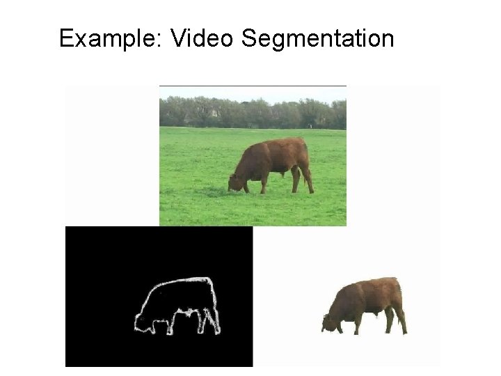
Example: Video Segmentation

Model Based Segmentation Image Segmentation Pose Estimate [Images courtesy: M. Black, L. Sigal]

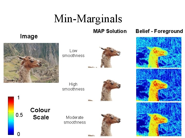
Min-Marginals MAP Solution Image Low smoothness High smoothness 1 0. 5 0 Colour Scale Moderate smoothness Belief - Foreground

Uses of Min marginals • Estimate of true marginals (uncertainty) • Parameter Learning. • Get best n solutions easily.

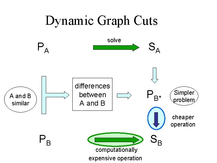
Dynamic Graph Cuts PA solve differences between A and B similar SA PB* Simpler problem cheaper operation PB computationally expensive operation SB

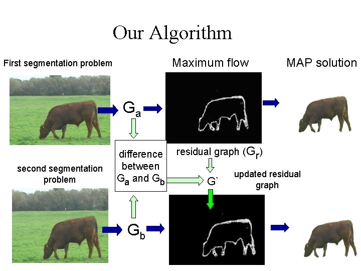
Our Algorithm Maximum flow First segmentation problem MAP solution Ga second segmentation problem difference between Ga and Gb Gb residual graph (Gr) G` updated residual graph

Computing the st-mincut from Max-flow algorithms • The Max-flow Problem - Edge capacity and flow balance constraints • Notation - Residual capacity (edge capacity – current flow) - Augmenting path Source (0) 2 1 a 1 • Simple Augmenting Path based Algorithms - Repeatedly find augmenting paths and push flow. - Saturated edges constitute the st-mincut. [Ford-Fulkerson Theorem] 9 a 2 2 5 4 Sink (1)

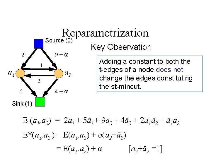
Reparametrization Source (0) 9+α 2 1 a 1 2 5 a 2 4+α Key Observation Adding a constant to both the t-edges of a node does not change the edges constituting the st-mincut. Sink (1) E (a 1, a 2) = 2 a 1 + 5ā1+ 9 a 2 + 4ā2 + 2 a 1ā2 + ā1 a 2 E*(a 1, a 2 ) = E(a 1, a 2) + α(a 2+ā2) = E(a 1, a 2) + α [a 2+ā2 =1]

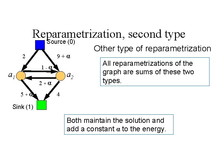
Reparametrization, second type Source (0) 9+α 2 1 -α a 1 a 2 2+α 5+α Other type of reparametrization All reparametrizations of the graph are sums of these two types. 4 Sink (1) Both maintain the solution and add a constant α to the energy.

Reparametrization • Nice result (easy to prove) • All other reparametrizations can be viewed in terms of these two basic operations. • Proof in Hammer, and also in one of Vlad’s recent papers.

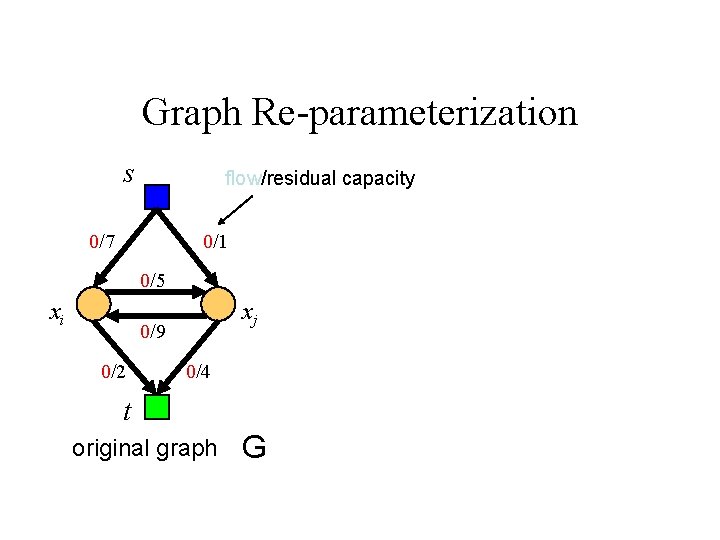
Graph Re-parameterization s flow/residual capacity 0/7 0/1 0/5 xi xj 0/9 0/2 0/4 t original graph G

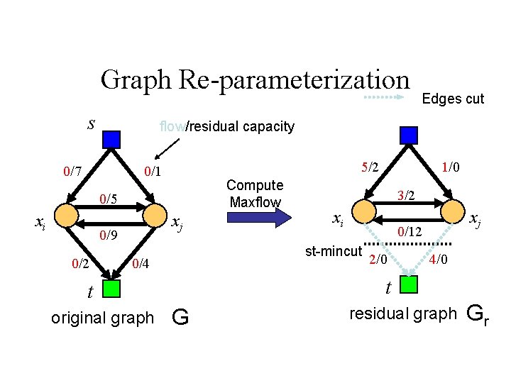
Graph Re-parameterization s flow/residual capacity 0/7 5/2 0/1 Compute Maxflow 0/5 xi xj 0/9 0/2 Edges cut xi xj 0/12 2/0 4/0 t t original graph 3/2 st-mincut 0/4 1/0 G residual graph Gr

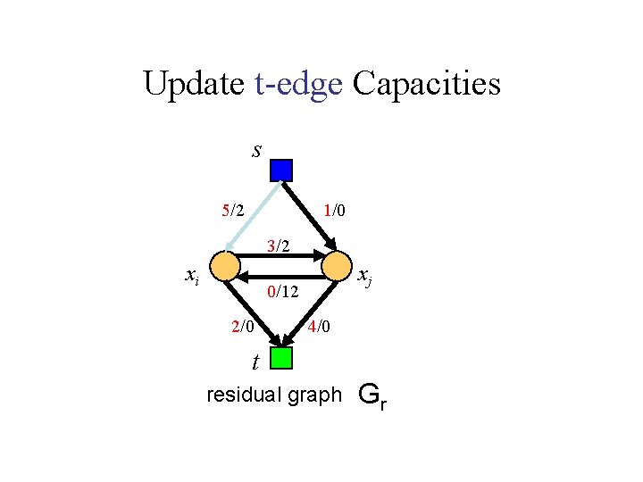
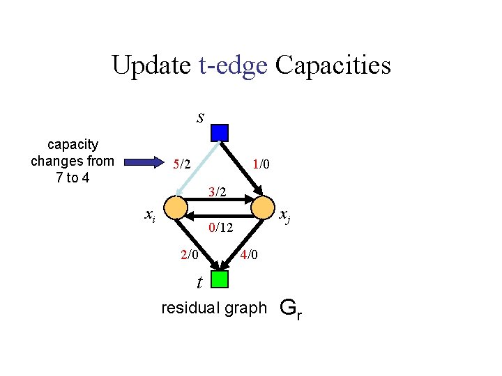
Update t-edge Capacities s 5/2 1/0 3/2 xi xj 0/12 2/0 4/0 t residual graph Gr

Update t-edge Capacities s capacity changes from 7 to 4 5/2 1/0 3/2 xi xj 0/12 2/0 4/0 t residual graph Gr

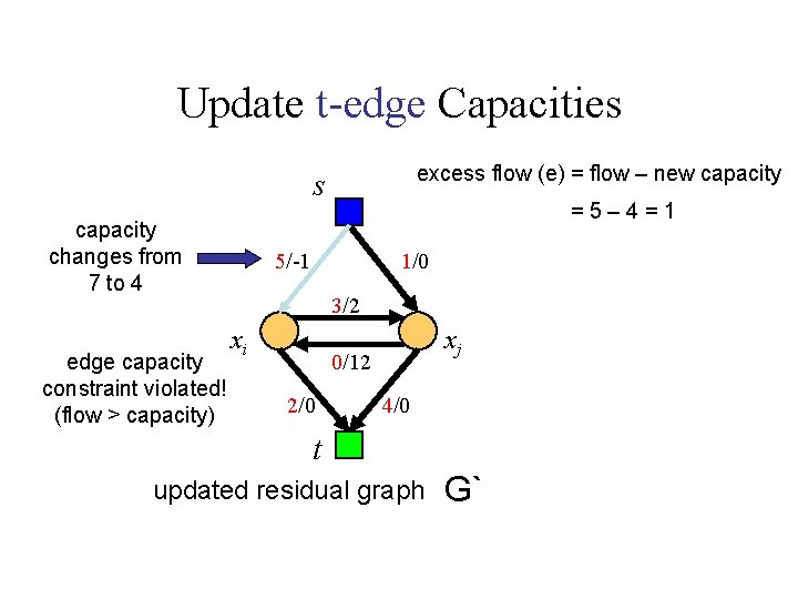
Update t-edge Capacities excess flow (e) = flow – new capacity s capacity changes from 7 to 4 edge capacity constraint violated! (flow > capacity) =5– 4=1 5/-1 1/0 3/2 xi xj 0/12 2/0 4/0 t updated residual graph G`

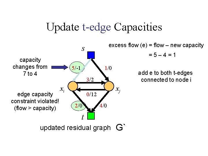
Update t-edge Capacities excess flow (e) = flow – new capacity s capacity changes from 7 to 4 edge capacity constraint violated! (flow > capacity) =5– 4=1 5/-1 1/0 add e to both t-edges connected to node i 3/2 xi xj 0/12 2/0 4/0 t updated residual graph G`

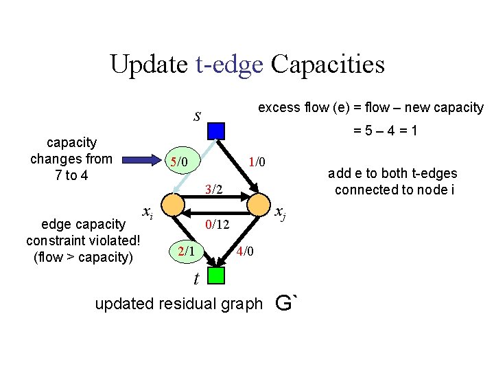
Update t-edge Capacities excess flow (e) = flow – new capacity s capacity changes from 7 to 4 edge capacity constraint violated! (flow > capacity) =5– 4=1 5/0 1/0 add e to both t-edges connected to node i 3/2 xi xj 0/12 2/1 4/0 t updated residual graph G`

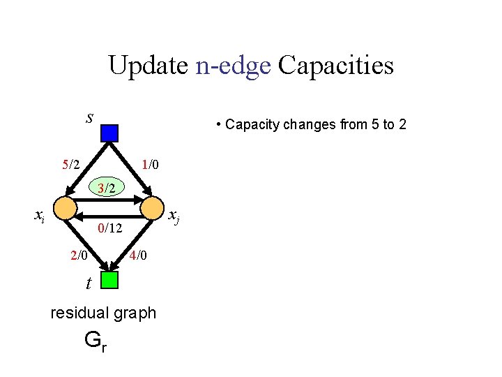
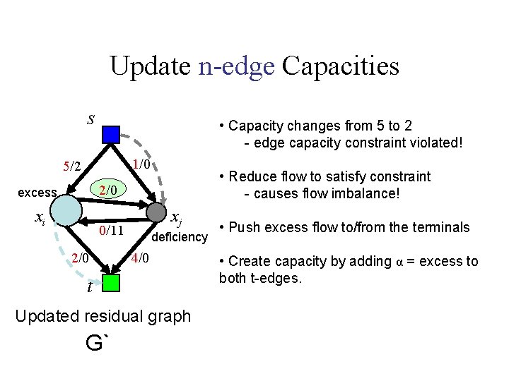
Update n-edge Capacities s • Capacity changes from 5 to 2 5/2 1/0 3/2 xi xj 0/12 2/0 4/0 t residual graph Gr

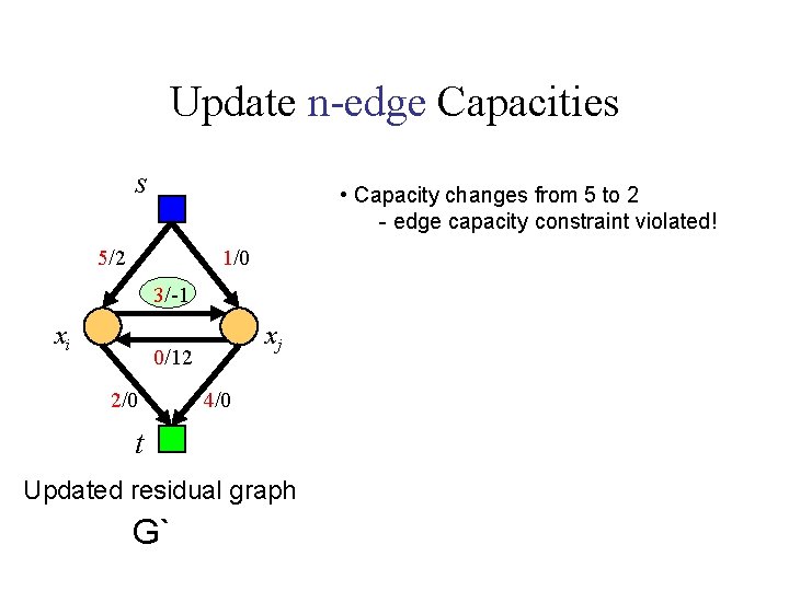
Update n-edge Capacities s • Capacity changes from 5 to 2 - edge capacity constraint violated! 5/2 1/0 3/-1 xi xj 0/12 2/0 4/0 t Updated residual graph G`

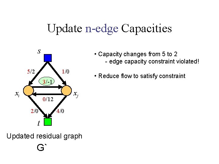
Update n-edge Capacities s • Capacity changes from 5 to 2 - edge capacity constraint violated! 5/2 1/0 • Reduce flow to satisfy constraint 3/-1 xi xj 0/12 2/0 4/0 t Updated residual graph G`

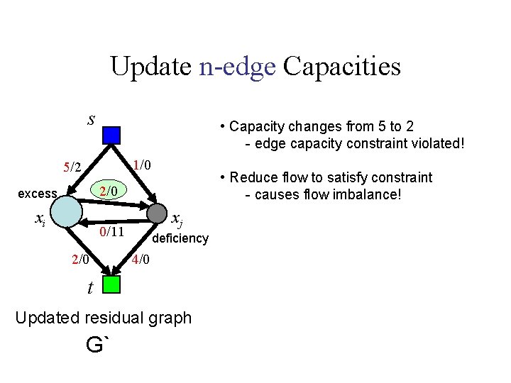
Update n-edge Capacities s • Capacity changes from 5 to 2 - edge capacity constraint violated! 1/0 5/2 • Reduce flow to satisfy constraint - causes flow imbalance! 2/0 excess xi xj 0/11 2/0 deficiency 4/0 t Updated residual graph G`

Update n-edge Capacities s • Capacity changes from 5 to 2 - edge capacity constraint violated! 1/0 5/2 • Reduce flow to satisfy constraint - causes flow imbalance! 2/0 excess xi xj 0/11 2/0 deficiency 4/0 t Updated residual graph G` • Push excess flow to/from the terminals • Create capacity by adding α = excess to both t-edges.

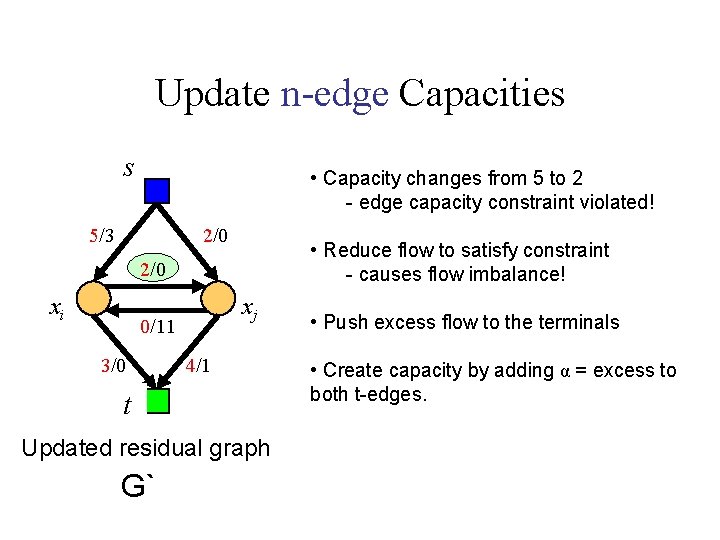
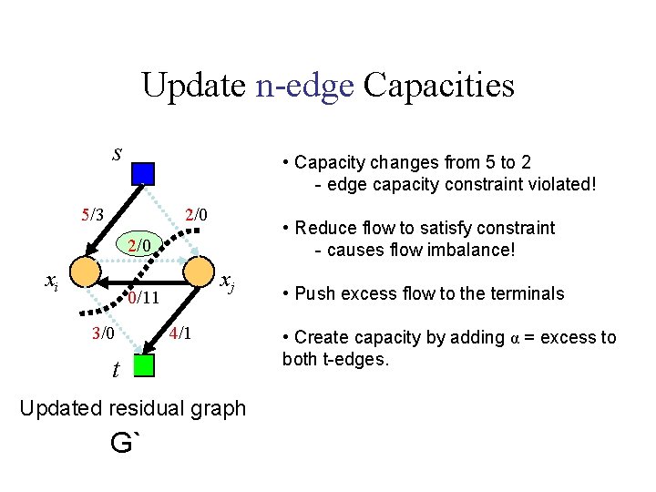
Update n-edge Capacities s • Capacity changes from 5 to 2 - edge capacity constraint violated! 5/3 2/0 • Reduce flow to satisfy constraint - causes flow imbalance! 2/0 xi xj 0/11 3/0 4/1 t Updated residual graph G` • Push excess flow to the terminals • Create capacity by adding α = excess to both t-edges.

Update n-edge Capacities s • Capacity changes from 5 to 2 - edge capacity constraint violated! 5/3 2/0 • Reduce flow to satisfy constraint - causes flow imbalance! 2/0 xi xj 0/11 3/0 4/1 t Updated residual graph G` • Push excess flow to the terminals • Create capacity by adding α = excess to both t-edges.

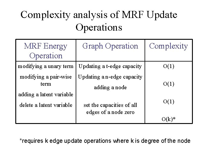
Complexity analysis of MRF Update Operations MRF Energy Operation Graph Operation modifying a unary term Updating a t-edge capacity modifying a pair-wise term Complexity O(1) Updating a n-edge capacity adding a node O(1) adding a latent variable delete a latent variable set the capacities of all edges of a node zero O(1) O(k)* *requires k edge update operations where k is degree of the node

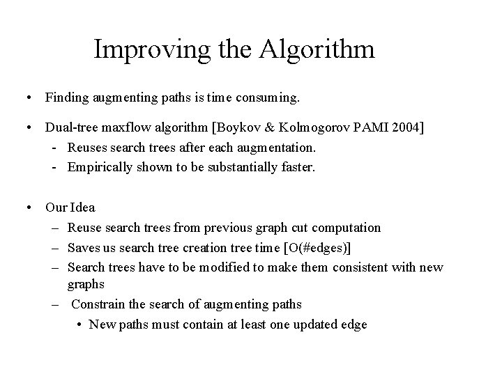
Improving the Algorithm • Finding augmenting paths is time consuming. • Dual-tree maxflow algorithm [Boykov & Kolmogorov PAMI 2004] - Reuses search trees after each augmentation. - Empirically shown to be substantially faster. • Our Idea – Reuse search trees from previous graph cut computation – Saves us search tree creation tree time [O(#edges)] – Search trees have to be modified to make them consistent with new graphs – Constrain the search of augmenting paths • New paths must contain at least one updated edge

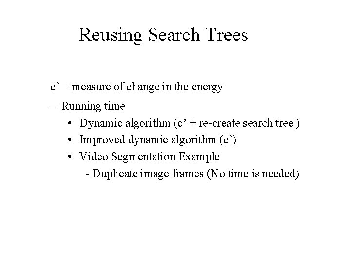
Reusing Search Trees c’ = measure of change in the energy – Running time • Dynamic algorithm (c’ + re-create search tree ) • Improved dynamic algorithm (c’) • Video Segmentation Example - Duplicate image frames (No time is needed)

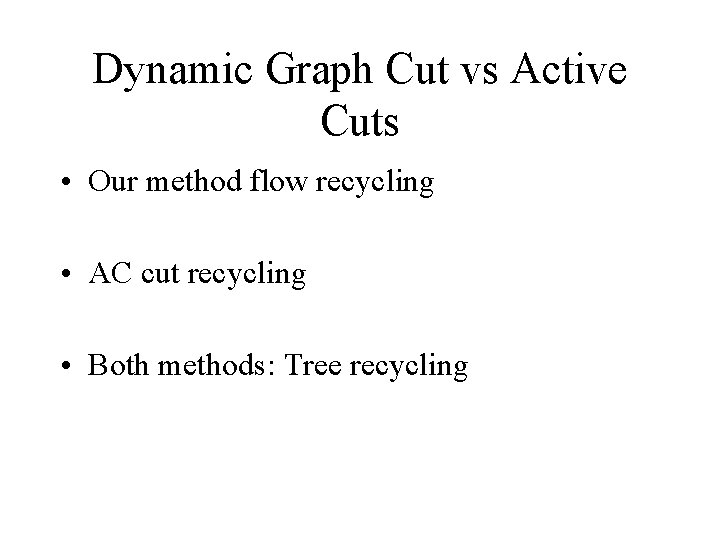
Dynamic Graph Cut vs Active Cuts • Our method flow recycling • AC cut recycling • Both methods: Tree recycling

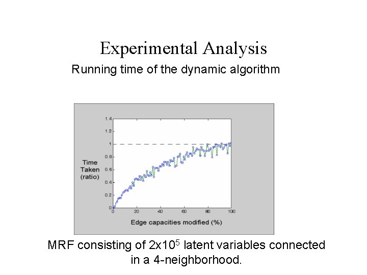
Experimental Analysis Running time of the dynamic algorithm MRF consisting of 2 x 105 latent variables connected in a 4 -neighborhood.

Part II SOCP for MRF

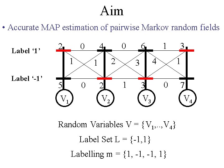
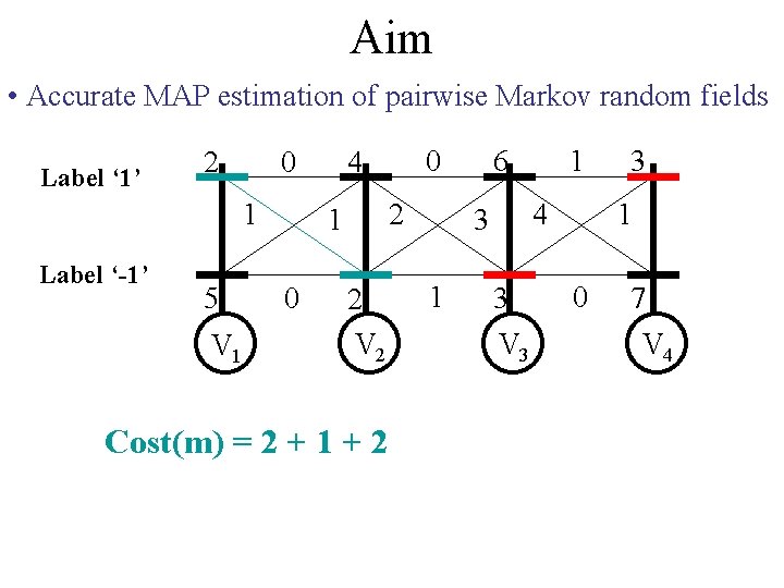
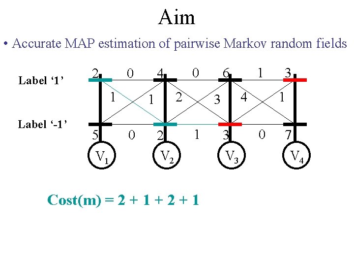
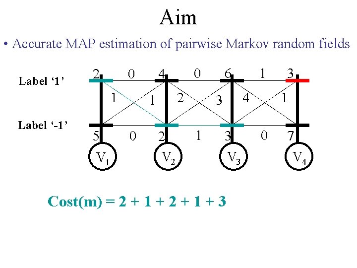
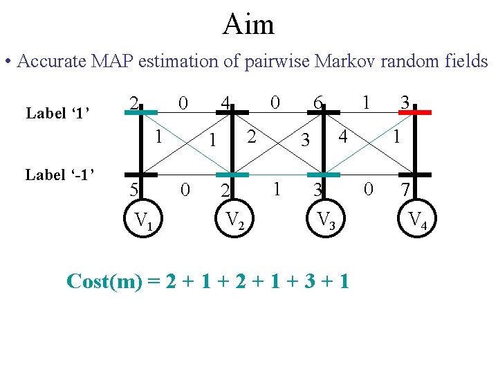
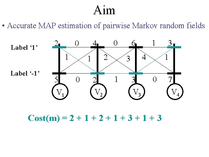
Aim • Accurate MAP estimation of pairwise Markov random fields Label ‘ 1’ 2 0 1 Label ‘-1’ 5 V 1 2 1 0 0 4 2 V 2 6 4 3 1 1 3 3 1 0 V 3 Random Variables V = {V 1, . . , V 4} Label Set L = {-1, 1} Labelling m = {1, -1, 1} 7 V 4

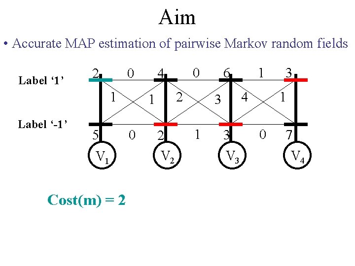
Aim • Accurate MAP estimation of pairwise Markov random fields Label ‘ 1’ 2 0 1 Label ‘-1’ 5 V 1 Cost(m) = 2 2 1 0 0 4 2 V 2 6 4 3 1 1 3 V 3 3 1 0 7 V 4

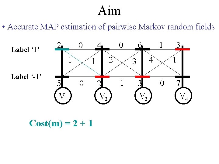
Aim • Accurate MAP estimation of pairwise Markov random fields Label ‘ 1’ 2 0 1 Label ‘-1’ 5 0 4 2 1 0 V 1 Cost(m) = 2 + 1 2 V 2 6 4 3 1 1 3 V 3 3 1 0 7 V 4

Aim • Accurate MAP estimation of pairwise Markov random fields Label ‘ 1’ 2 0 1 Label ‘-1’ 5 V 1 2 1 0 0 4 2 V 2 Cost(m) = 2 + 1 + 2 6 4 3 1 1 3 V 3 3 1 0 7 V 4

Aim • Accurate MAP estimation of pairwise Markov random fields Label ‘ 1’ 2 0 1 Label ‘-1’ 5 V 1 2 1 0 0 4 2 V 2 6 4 3 1 Cost(m) = 2 + 1 + 2 + 1 1 3 V 3 3 1 0 7 V 4

Aim • Accurate MAP estimation of pairwise Markov random fields Label ‘ 1’ 2 0 1 Label ‘-1’ 5 V 1 2 1 0 0 4 2 V 2 6 4 3 1 1 3 Cost(m) = 2 + 1 + 3 V 3 3 1 0 7 V 4

Aim • Accurate MAP estimation of pairwise Markov random fields Label ‘ 1’ 2 0 1 Label ‘-1’ 5 V 1 2 1 0 0 4 2 V 2 6 4 3 1 1 3 V 3 Cost(m) = 2 + 1 + 3 + 1 3 1 0 7 V 4

Aim • Accurate MAP estimation of pairwise Markov random fields Label ‘ 1’ 2 0 1 Label ‘-1’ 5 V 1 2 1 0 0 4 2 V 2 6 4 3 1 1 3 3 1 0 V 3 Cost(m) = 2 + 1 + 3 7 V 4

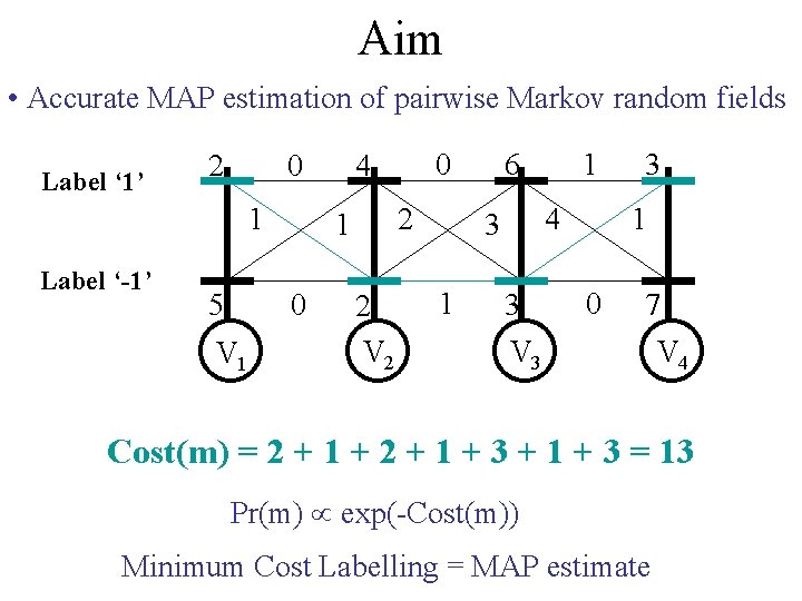
Aim • Accurate MAP estimation of pairwise Markov random fields Label ‘ 1’ 2 0 1 Label ‘-1’ 5 V 1 2 1 0 0 4 2 V 2 6 4 3 1 1 3 3 1 0 7 V 3 V 4 Cost(m) = 2 + 1 + 3 = 13 Pr(m) exp(-Cost(m)) Minimum Cost Labelling = MAP estimate

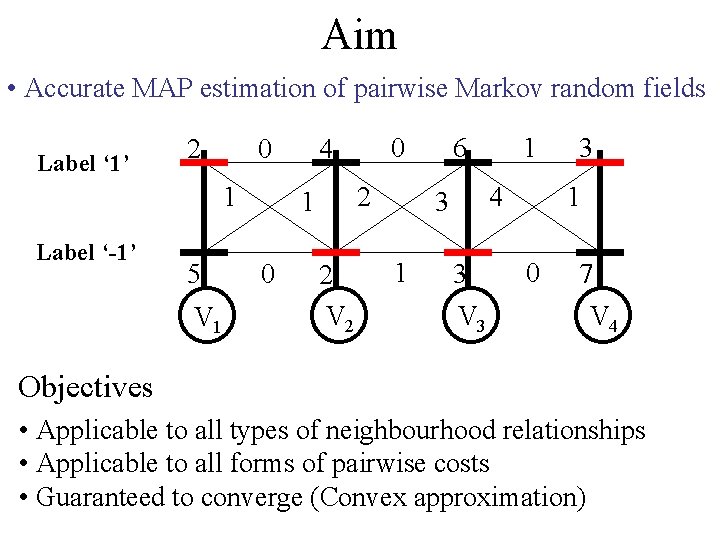
Aim • Accurate MAP estimation of pairwise Markov random fields Label ‘ 1’ 2 0 1 Label ‘-1’ 5 V 1 2 1 0 0 4 2 V 2 6 4 3 1 1 3 V 3 3 1 0 7 V 4 Objectives • Applicable to all types of neighbourhood relationships • Applicable to all forms of pairwise costs • Guaranteed to converge (Convex approximation)

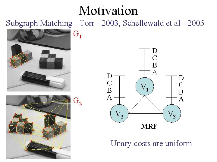
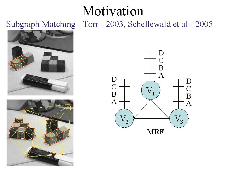
Motivation Subgraph Matching - Torr - 2003, Schellewald et al - 2005 G 1 G 2 D C B A V 1 V 2 V 3 MRF Unary costs are uniform

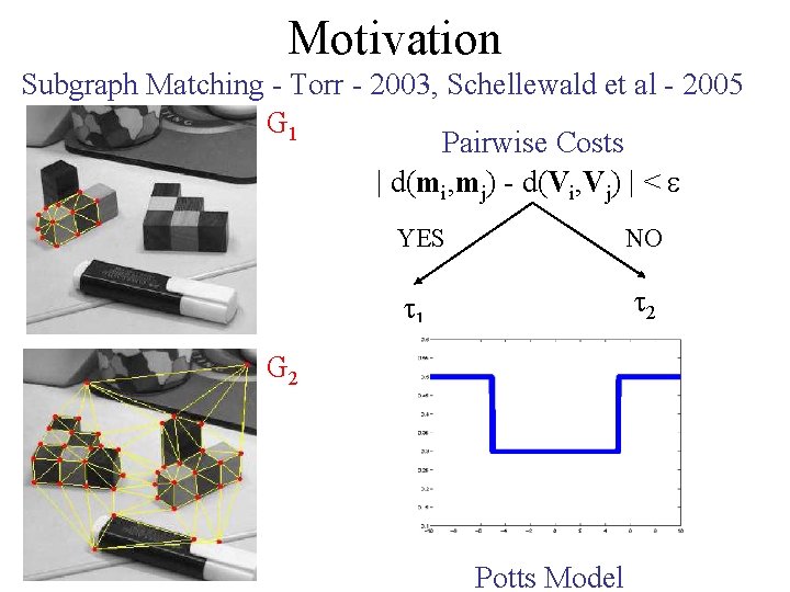
Motivation Subgraph Matching - Torr - 2003, Schellewald et al - 2005 G 1 Pairwise Costs | d(mi, mj) - d(Vi, Vj) | < YES NO 1 2 G 2 Potts Model

Motivation Subgraph Matching - Torr - 2003, Schellewald et al - 2005 D C B A V 1 V 2 V 3 MRF

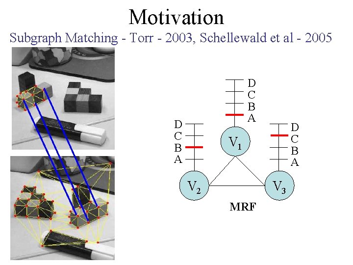
Motivation Subgraph Matching - Torr - 2003, Schellewald et al - 2005 D C B A V 1 V 2 V 3 MRF

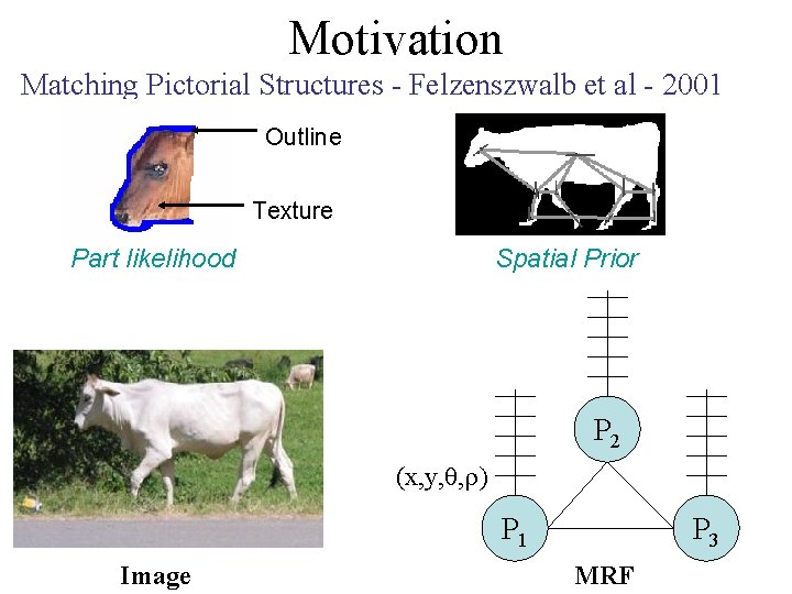
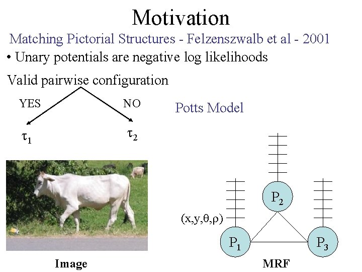
Motivation Matching Pictorial Structures - Felzenszwalb et al - 2001 Outline Texture Part likelihood Spatial Prior P 2 (x, y, , ) P 1 Image P 3 MRF

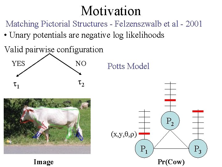
Motivation Matching Pictorial Structures - Felzenszwalb et al - 2001 • Unary potentials are negative log likelihoods Valid pairwise configuration YES NO 1 2 Potts Model P 2 (x, y, , ) P 1 Image P 3 MRF

Motivation Matching Pictorial Structures - Felzenszwalb et al - 2001 • Unary potentials are negative log likelihoods Valid pairwise configuration YES NO 1 2 Potts Model P 2 (x, y, , ) P 1 Image P 3 Pr(Cow)

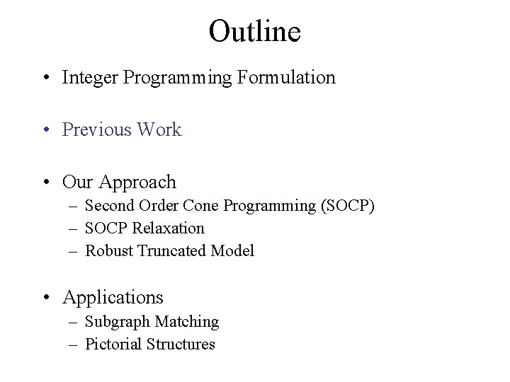
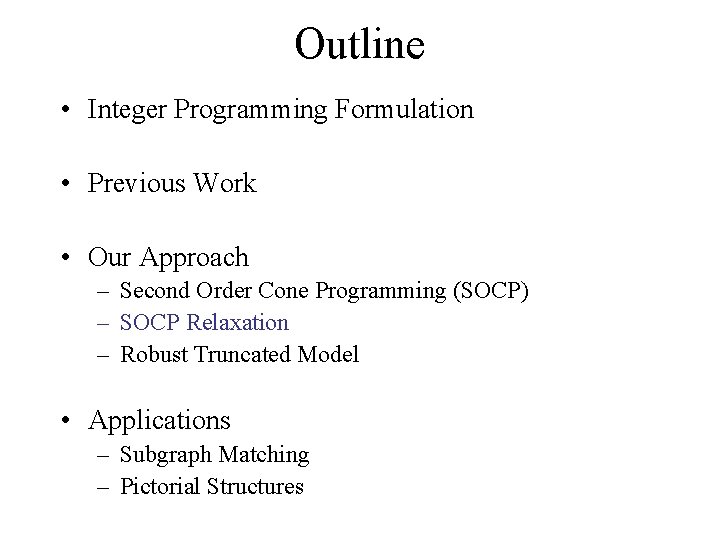
Outline • Integer Programming Formulation • Previous Work • Our Approach – Second Order Cone Programming (SOCP) – SOCP Relaxation – Robust Truncated Model • Applications – Subgraph Matching – Pictorial Structures

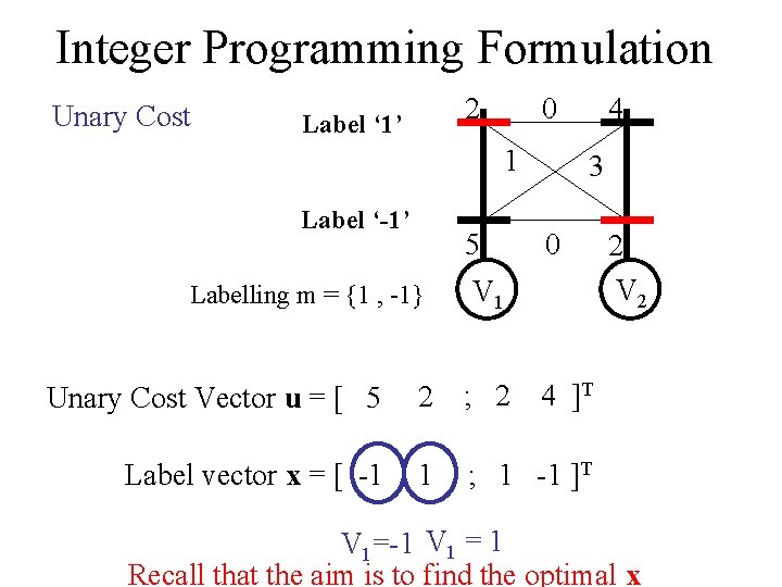
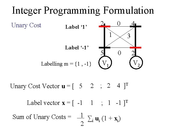
Integer Programming Formulation Unary Cost 2 Label ‘ 1’ 0 1 Label ‘-1’ 5 Labelling m = {1 , -1} 4 3 0 V 1 Unary Cost Vector u = [ 5 2 ; 2 Label vector x = [ -1 1 ; 1 -1 ]T 2 V 2 4 ]T V 1=-1 V 1 = 1 Recall that the aim is to find the optimal x

Integer Programming Formulation Unary Cost 2 Label ‘ 1’ 0 1 Label ‘-1’ 5 Labelling m = {1 , -1} 4 3 0 V 1 Unary Cost Vector u = [ 5 2 ; 2 Label vector x = [ -1 1 ; 1 -1 ]T Sum of Unary Costs = 4 ]T 1 ∑ u (1 + x ) i i i 2 2 V 2

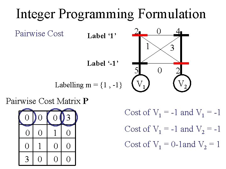
Integer Programming Formulation Pairwise Cost Label ‘ 1’ 2 0 1 Label ‘-1’ Labelling m = {1 , -1} 5 V 1 4 3 0 2 V 2 Pairwise Cost Matrix P 0 0 0 3 0 0 0 1 1 0 0 0 3 0 0 0 Cost of V 1 = -1 and V 1 = -1 Cost of V 1 = -1 and V 2 = -1 Cost of V 1 = 0 -1 and V 2 = 1

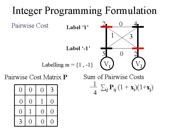
Integer Programming Formulation Pairwise Cost Label ‘ 1’ 2 0 1 Label ‘-1’ Labelling m = {1 , -1} Pairwise Cost Matrix P 0 0 0 3 0 0 0 1 1 0 0 0 3 0 0 0 5 V 1 4 3 0 2 V 2 Sum of Pairwise Costs 1 ∑ P (1 + x )(1+x ) ij ij i j 4

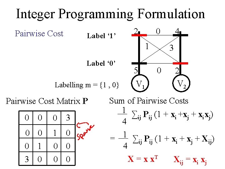
Integer Programming Formulation Pairwise Cost Label ‘ 1’ 2 0 1 Label ‘ 0’ Labelling m = {1 , 0} Pairwise Cost Matrix P 0 0 0 3 0 0 0 1 1 0 0 0 3 0 0 0 5 V 1 4 3 0 2 V 2 Sum of Pairwise Costs 1 ∑ P (1 + x +x + x x ) ij ij i j 4 = 1 ∑ij Pij (1 + xi + xj + Xij) 4 X = x x. T Xij = xi xj

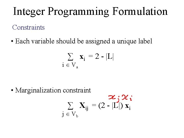
Integer Programming Formulation Constraints • Each variable should be assigned a unique label ∑ xi = 2 - |L| i Va • Marginalization constraint ∑ Xij = (2 - |L|) xi j Vb

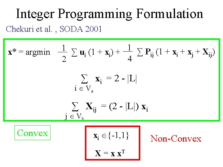
Integer Programming Formulation Chekuri et al. , SODA 2001 x* = argmin 1 ∑ u (1 + x ) + 1 ∑ P (1 + x + X ) ij i j ij i i 4 2 ∑ xi = 2 - |L| i Va ∑ Xij = (2 - |L|) xi j Vb Convex xi {-1, 1} X = x x. T Non-Convex

Key Point • In modern optimization the issue is not linear vs non linear but convex vs nonconvex • We want to find a convex and good relaxation of the integer program.

Outline • Integer Programming Formulation • Previous Work • Our Approach – Second Order Cone Programming (SOCP) – SOCP Relaxation – Robust Truncated Model • Applications – Subgraph Matching – Pictorial Structures

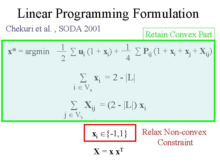
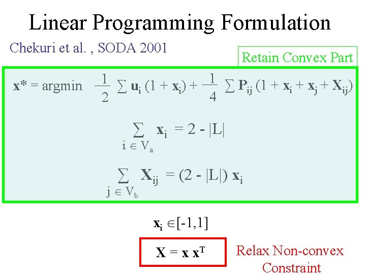
Linear Programming Formulation Chekuri et al. , SODA 2001 x* = argmin Retain Convex Part 1 ∑ u (1 + x ) + 1 ∑ P (1 + x + X ) ij i j ij i i 4 2 ∑ xi = 2 - |L| i Va ∑ Xij = (2 - |L|) xi j Vb xi {-1, 1} X = x x. T Relax Non-convex Constraint

Linear Programming Formulation Chekuri et al. , SODA 2001 x* = argmin Retain Convex Part 1 ∑ u (1 + x ) + 1 ∑ P (1 + x + X ) ij i j ij i i 4 2 ∑ xi = 2 - |L| i Va ∑ Xij = (2 - |L|) xi j Vb xi [-1, 1] X = x x. T Relax Non-convex Constraint

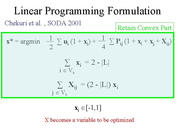
Linear Programming Formulation Chekuri et al. , SODA 2001 x* = argmin Retain Convex Part 1 ∑ u (1 + x ) + 1 ∑ P (1 + x + X ) ij i j ij i i 4 2 ∑ xi = 2 - |L| i Va ∑ Xij = (2 - |L|) xi j Vb xi [-1, 1] X becomes a variable to be optimized

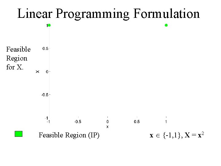
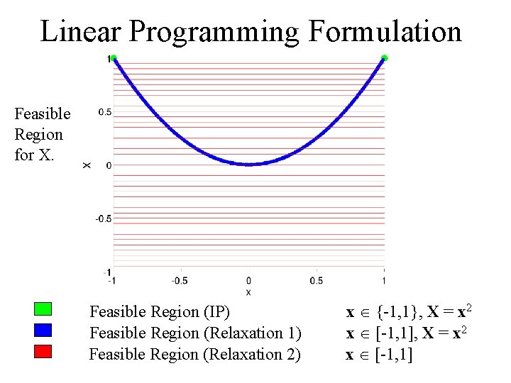
Linear Programming Formulation Feasible Region for X. Feasible Region (IP) x {-1, 1}, X = x 2

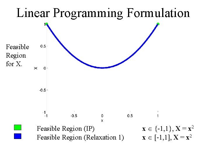
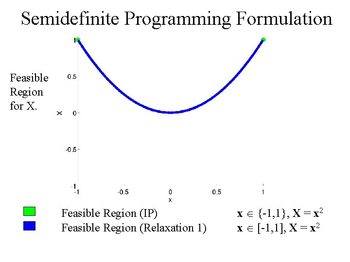
Linear Programming Formulation Feasible Region for X. Feasible Region (IP) Feasible Region (Relaxation 1) x {-1, 1}, X = x 2 x [-1, 1], X = x 2

Linear Programming Formulation Feasible Region for X. Feasible Region (IP) Feasible Region (Relaxation 1) Feasible Region (Relaxation 2) x {-1, 1}, X = x 2 x [-1, 1]

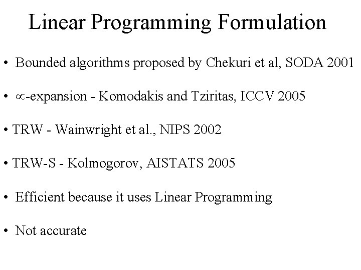
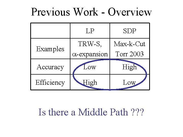
Linear Programming Formulation • Bounded algorithms proposed by Chekuri et al, SODA 2001 • -expansion - Komodakis and Tziritas, ICCV 2005 • TRW - Wainwright et al. , NIPS 2002 • TRW-S - Kolmogorov, AISTATS 2005 • Efficient because it uses Linear Programming • Not accurate

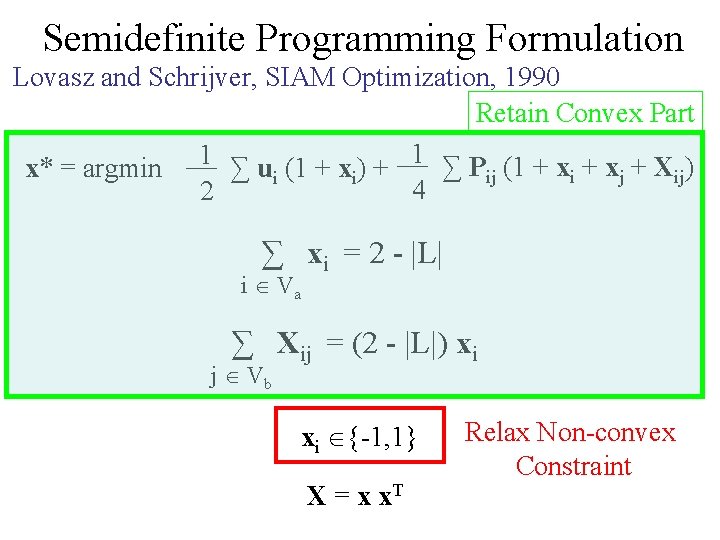
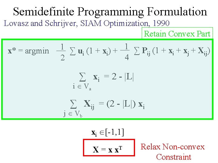
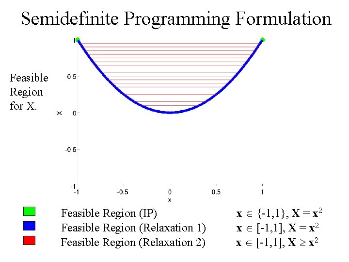
Semidefinite Programming Formulation Lovasz and Schrijver, SIAM Optimization, 1990 Retain Convex Part 1 ∑ P (1 + x + X ) 1 x* = argmin ∑ ui (1 + xi) + ij i j ij 4 2 ∑ xi = 2 - |L| i Va ∑ Xij = (2 - |L|) xi j Vb xi {-1, 1} X = x x. T Relax Non-convex Constraint

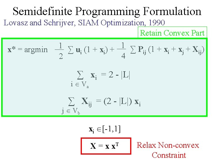
Semidefinite Programming Formulation Lovasz and Schrijver, SIAM Optimization, 1990 Retain Convex Part 1 ∑ P (1 + x + X ) 1 x* = argmin ∑ ui (1 + xi) + ij i j ij 4 2 ∑ xi = 2 - |L| i Va ∑ Xij = (2 - |L|) xi j Vb xi [-1, 1] X = x x. T Relax Non-convex Constraint

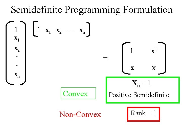
Semidefinite Programming Formulation 1 x 1 x 2 . . . xn . . . = xn 1 x. T x X Xii = 1 Convex Non-Convex Positive Semidefinite Rank = 1

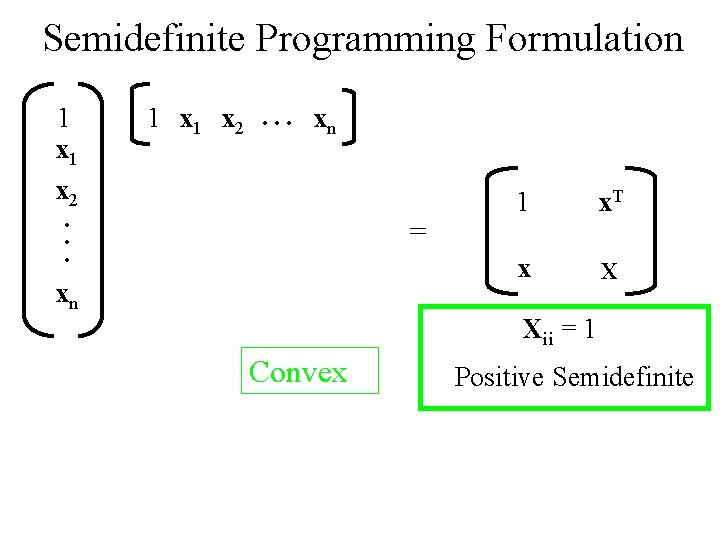
Semidefinite Programming Formulation 1 x 1 x 2 . . . xn . . . = xn 1 x. T x X Xii = 1 Convex Positive Semidefinite

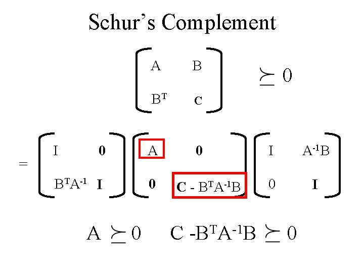
Schur’s Complement = I A B BT C 0 A BTA-1 I 0 A 0 0 C - BTA-1 B C -BTA-1 B 0 I 0

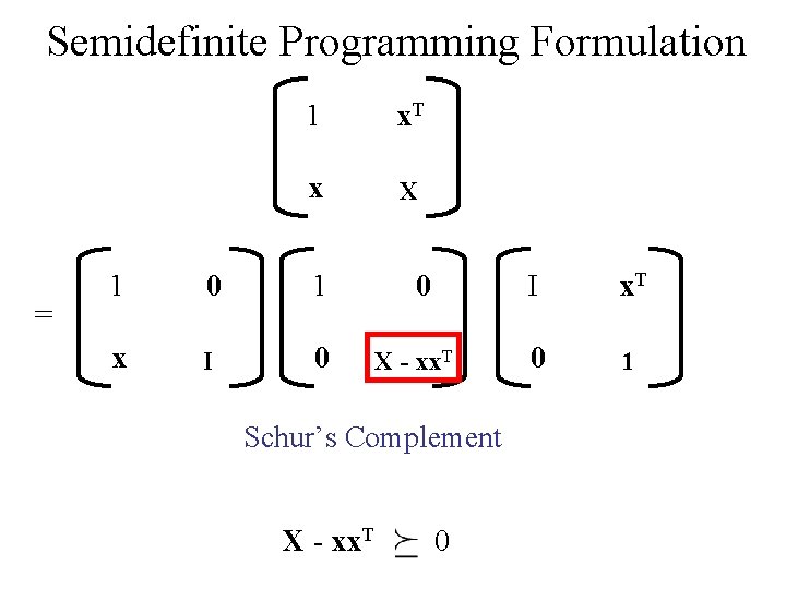
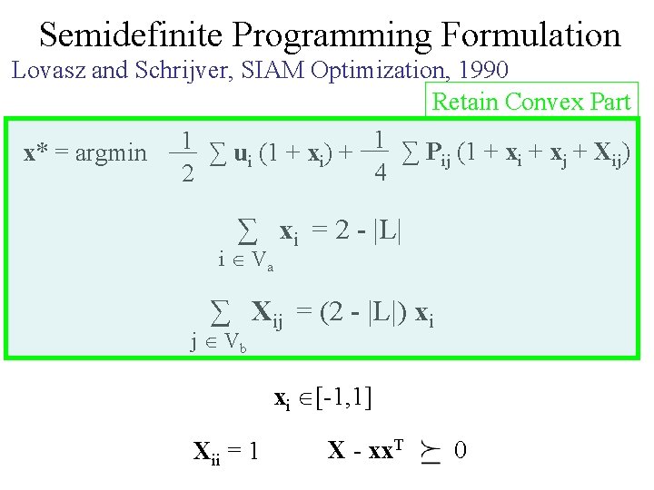
Semidefinite Programming Formulation = 1 x. T x X 1 0 1 x I 0 0 X - xx. T Schur’s Complement X - xx. T 0 I x. T 0 1

Semidefinite Programming Formulation Lovasz and Schrijver, SIAM Optimization, 1990 Retain Convex Part 1 ∑ P (1 + x + X ) 1 x* = argmin ∑ ui (1 + xi) + ij i j ij 4 2 ∑ xi = 2 - |L| i Va ∑ Xij = (2 - |L|) xi j Vb xi [-1, 1] X = x x. T Relax Non-convex Constraint

Semidefinite Programming Formulation Lovasz and Schrijver, SIAM Optimization, 1990 Retain Convex Part 1 ∑ P (1 + x + X ) 1 x* = argmin ∑ ui (1 + xi) + ij i j ij 4 2 ∑ xi = 2 - |L| i Va ∑ Xij = (2 - |L|) xi j Vb xi [-1, 1] Xii = 1 X - xx. T 0

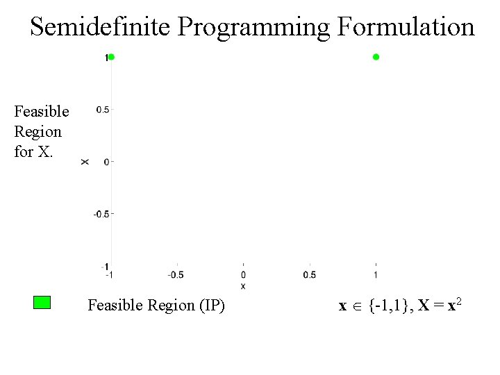
Semidefinite Programming Formulation Feasible Region for X. Feasible Region (IP) x {-1, 1}, X = x 2

Semidefinite Programming Formulation Feasible Region for X. Feasible Region (IP) Feasible Region (Relaxation 1) x {-1, 1}, X = x 2 x [-1, 1], X = x 2

Semidefinite Programming Formulation Feasible Region for X. Feasible Region (IP) Feasible Region (Relaxation 1) Feasible Region (Relaxation 2) x {-1, 1}, X = x 2 x [-1, 1], X x 2

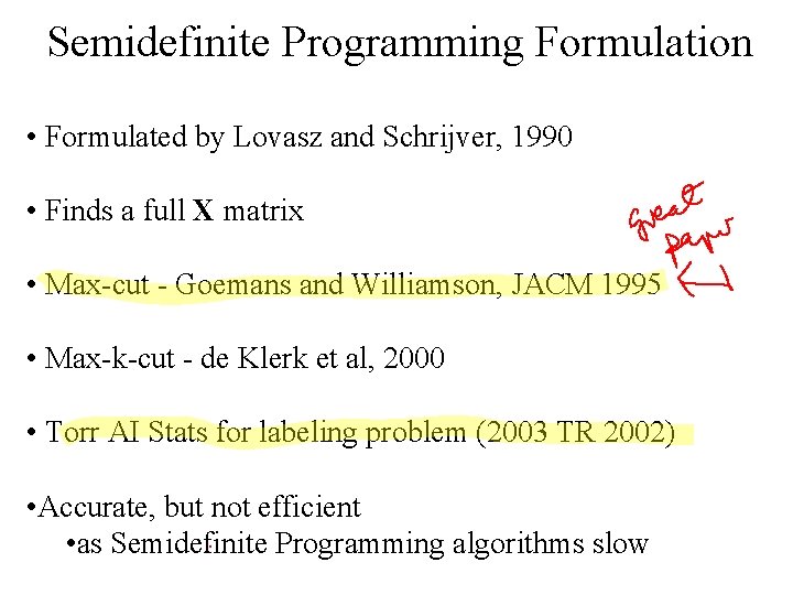
Semidefinite Programming Formulation • Formulated by Lovasz and Schrijver, 1990 • Finds a full X matrix • Max-cut - Goemans and Williamson, JACM 1995 • Max-k-cut - de Klerk et al, 2000 • Torr AI Stats for labeling problem (2003 TR 2002) • Accurate, but not efficient • as Semidefinite Programming algorithms slow

Previous Work - Overview LP Examples SDP TRW-S, Max-k-Cut -expansion Torr 2003 Accuracy Low High Efficiency High Low Is there a Middle Path ? ? ?

Outline • Integer Programming Formulation • Previous Work • Our Approach – Second Order Cone Programming (SOCP) – SOCP Relaxation – Robust Truncated Model • Applications – Subgraph Matching – Pictorial Structures

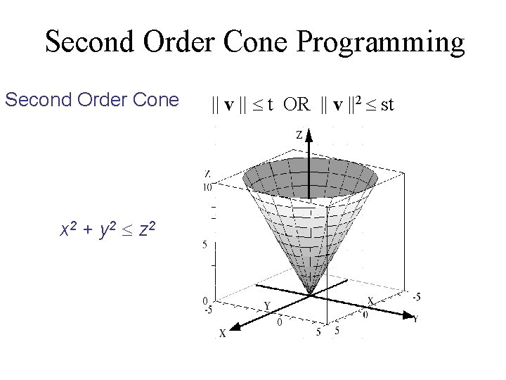
Second Order Cone Programming Second Order Cone x 2 + y 2 z 2 || v || t OR || v ||2 st

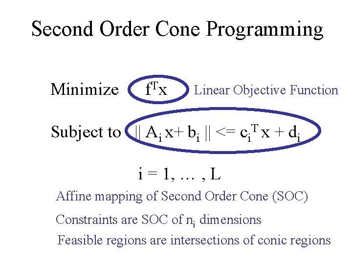
Second Order Cone Programming Minimize f. T x Linear Objective Function Subject to || Ai x+ bi || <= ci. T x + di i = 1, … , L Affine mapping of Second Order Cone (SOC) Constraints are SOC of ni dimensions Feasible regions are intersections of conic regions

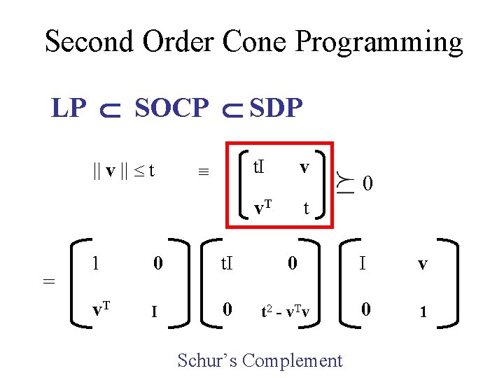
Second Order Cone Programming LP SOCP SDP || v || t = 1 0 t. I v. T I 0 t. I v v. T t 0 t 2 - v. Tv Schur’s Complement 0 I v 0 1

Outline • Integer Programming Formulation • Previous Work • Our Approach – Second Order Cone Programming (SOCP) – SOCP Relaxation – Robust Truncated Model • Applications – Subgraph Matching – Pictorial Structures

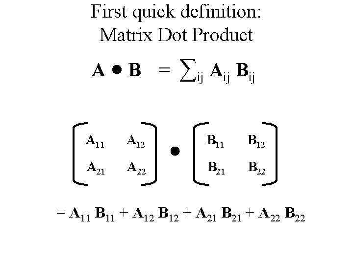
First quick definition: Matrix Dot Product A B = ∑ij Aij Bij A 11 A 12 B 11 B 12 A 21 A 22 B 21 B 22 = A 11 B 11 + A 12 B 12 + A 21 B 21 + A 22 B 22

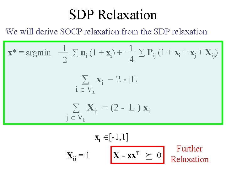
SDP Relaxation We will derive SOCP relaxation from the SDP relaxation x* = argmin 1 ∑ u (1 + x ) + 1 ∑ P (1 + x + X ) ij i j ij i i 4 2 ∑ xi = 2 - |L| i Va ∑ Xij = (2 - |L|) xi j Vb xi [-1, 1] Xii = 1 X- xx. T 0 Further Relaxation

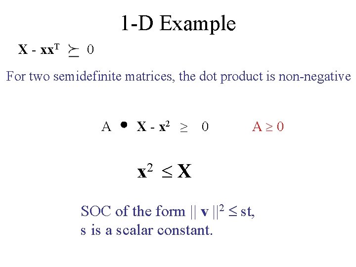
1 -D Example X - xx. T 0 For two semidefinite matrices, the dot product is non-negative A X - x 2 ≥ 0 A 0 x 2 X SOC of the form || v ||2 st, s is a scalar constant.

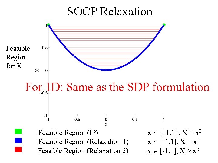
SOCP Relaxation Feasible Region for X. For 1 D: Same as the SDP formulation Feasible Region (IP) Feasible Region (Relaxation 1) Feasible Region (Relaxation 2) x {-1, 1}, X = x 2 x [-1, 1], X x 2

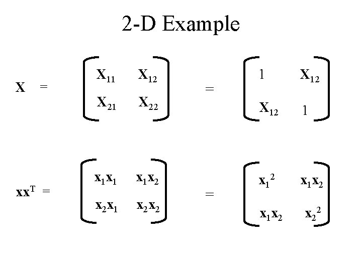
2 -D Example X = xx. T = X 11 X 12 X 21 X 22 x 1 x 1 x 1 x 2 x 2 x 1 x 2 x 2 = = 1 X 12 1 x 12 x 1 x 2 x 22

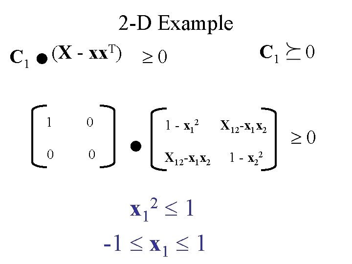
. C 1 2 -D Example (X - xx. T) 1 0 0 0 0 . 1 - x 12 X 12 -x 1 x 2 x 1 1 -1 x 1 1 2 C 1 X 12 -x 1 x 2 1 - x 2 2 0 0

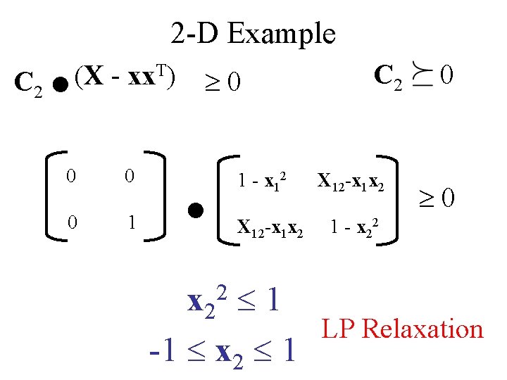
. C 2 2 -D Example (X - xx. T) 0 0 0 1 0 . 1 - x 12 X 12 -x 1 x 2 1 -1 x 2 1 C 2 X 12 -x 1 x 2 0 0 1 - x 2 2 2 LP Relaxation

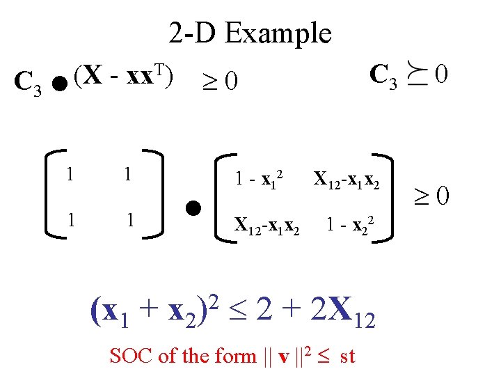
. C 3 2 -D Example (X - xx. T) 1 1 0 . 1 - x 12 X 12 -x 1 x 2 C 3 X 12 -x 1 x 2 1 - x 2 2 2 (x 1 + x 2) 2 + 2 X 12 SOC of the form || v ||2 st 0 0

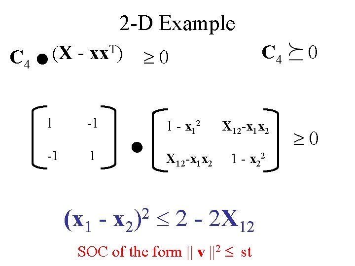
. C 4 2 -D Example (X - xx. T) 1 -1 -1 1 C 4 0 . 1 - x 12 X 12 -x 1 x 2 1 - x 2 2 2 (x 1 - x 2) 2 - 2 X 12 SOC of the form || v ||2 st 0 0

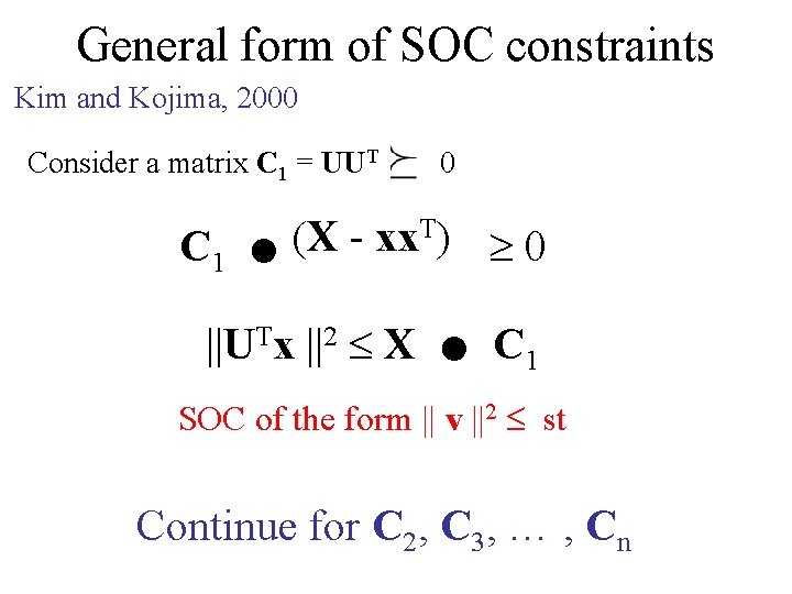
General form of SOC constraints . . Kim and Kojima, 2000 Consider a matrix C 1 = UUT C 1 0 (X - xx. T) 0 ||UTx ||2 X C 1 SOC of the form || v ||2 st Continue for C 2, C 3, … , Cn

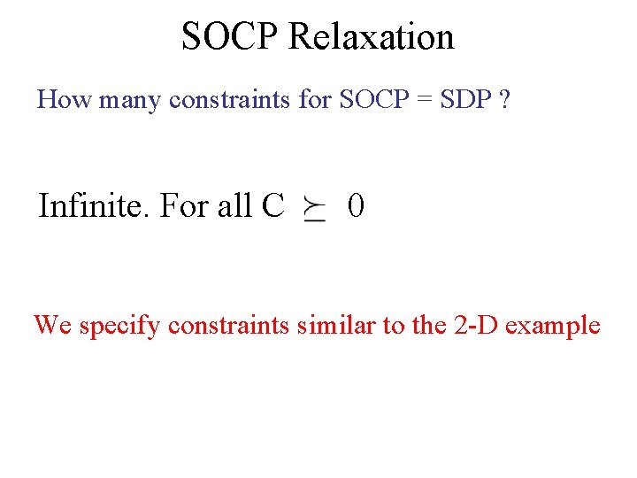
SOCP Relaxation How many constraints for SOCP = SDP ? Infinite. For all C 0 We specify constraints similar to the 2 -D example

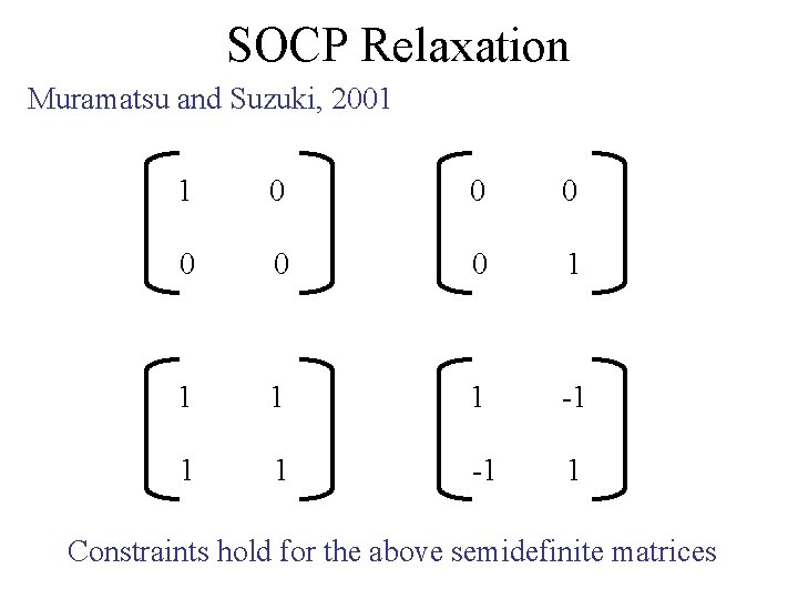
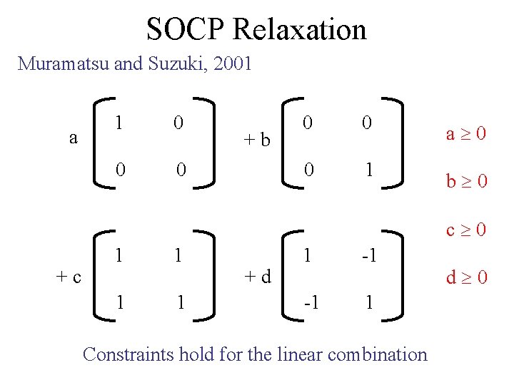
SOCP Relaxation Muramatsu and Suzuki, 2001 1 0 0 0 1 1 -1 1 Constraints hold for the above semidefinite matrices

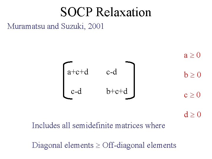
SOCP Relaxation Muramatsu and Suzuki, 2001 a 1 0 0 0 +b 0 0 a 0 0 1 b 0 c 0 +c 1 1 +d 1 -1 -1 1 Constraints hold for the linear combination d 0

SOCP Relaxation Muramatsu and Suzuki, 2001 a 0 a+c+d c-d b 0 b+c+d c 0 d 0 Includes all semidefinite matrices where Diagonal elements Off-diagonal elements

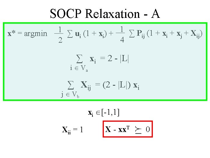
SOCP Relaxation - A x* = argmin 1 ∑ u (1 + x ) + 1 ∑ P (1 + x + X ) ij i j ij i i 4 2 ∑ xi = 2 - |L| i Va ∑ Xij = (2 - |L|) xi j Vb xi [-1, 1] Xii = 1 X - xx. T 0

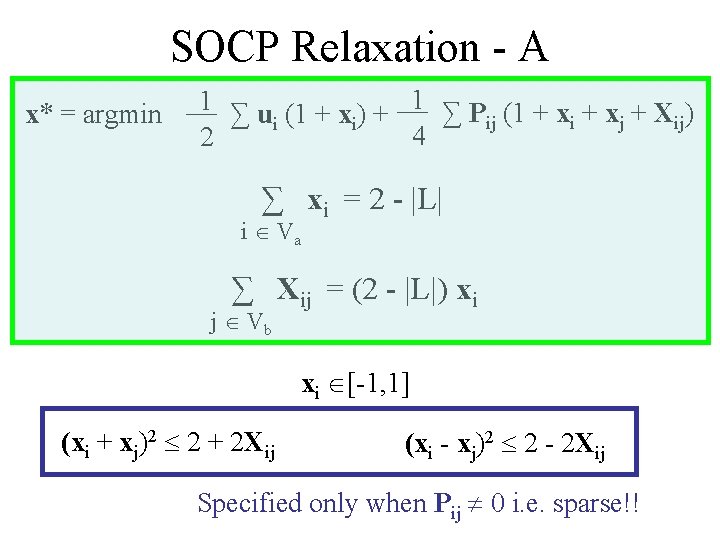
SOCP Relaxation - A x* = argmin 1 ∑ u (1 + x ) + 1 ∑ P (1 + x + X ) ij i j ij i i 4 2 ∑ xi = 2 - |L| i Va ∑ Xij = (2 - |L|) xi j Vb xi [-1, 1] (xi + xj)2 2 + 2 Xij (xi - xj)2 2 - 2 Xij Specified only when Pij 0 i. e. sparse!!

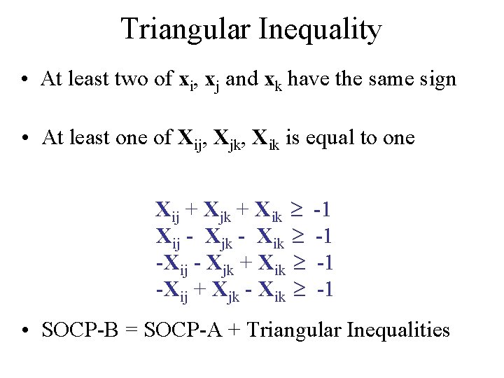
Triangular Inequality • At least two of xi, xj and xk have the same sign • At least one of Xij, Xjk, Xik is equal to one Xij + Xjk + Xik Xij - Xjk - Xik -Xij - Xjk + Xik -Xij + Xjk - Xik -1 -1 • SOCP-B = SOCP-A + Triangular Inequalities

Outline • Integer Programming Formulation • Previous Work • Our Approach – Second Order Cone Programming (SOCP) – SOCP Relaxation – Robust Truncated Model • Applications – Subgraph Matching – Pictorial Structures

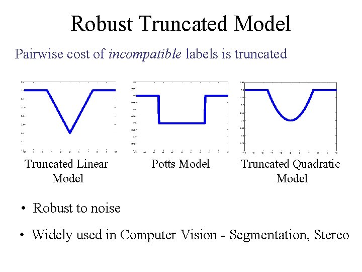
Robust Truncated Model Pairwise cost of incompatible labels is truncated Truncated Linear Model Potts Model Truncated Quadratic Model • Robust to noise • Widely used in Computer Vision - Segmentation, Stereo

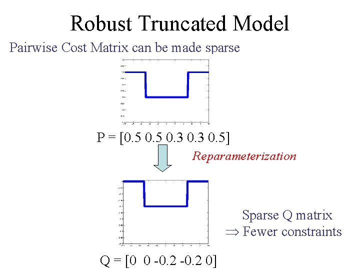
Robust Truncated Model Pairwise Cost Matrix can be made sparse P = [0. 5 0. 3 0. 5] Reparameterization Sparse Q matrix Fewer constraints Q = [0 0 -0. 2 0]

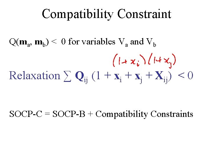
Compatibility Constraint Q(ma, mb) < 0 for variables Va and Vb Relaxation ∑ Qij (1 + xi + xj + Xij) < 0 SOCP-C = SOCP-B + Compatibility Constraints

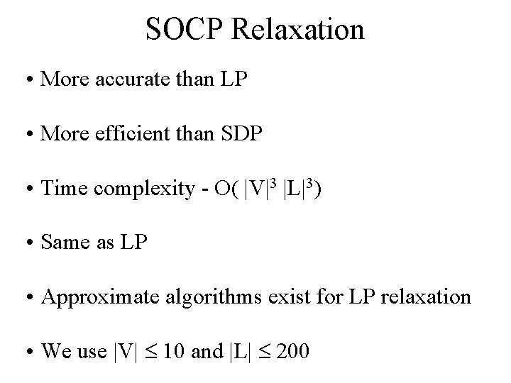
SOCP Relaxation • More accurate than LP • More efficient than SDP • Time complexity - O( |V|3 |L|3) • Same as LP • Approximate algorithms exist for LP relaxation • We use |V| 10 and |L| 200

Outline • Integer Programming Formulation • Previous Work • Our Approach – Second Order Cone Programming (SOCP) – SOCP Relaxation – Robust Truncated Model • Applications – Subgraph Matching – Pictorial Structures

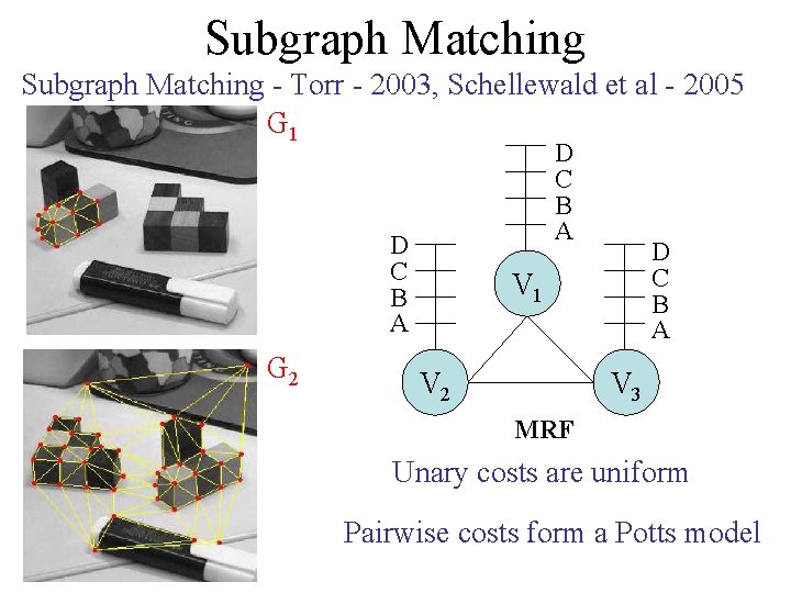
Subgraph Matching - Torr - 2003, Schellewald et al - 2005 G 1 D C B A G 2 D C B A V 1 V 2 V 3 MRF Unary costs are uniform Pairwise costs form a Potts model

Subgraph Matching • 1000 pairs of graphs G 1 and G 2 • #vertices in G 2 - between 20 and 30 • #vertices in G 1 - 0. 25 * #vertices in G 2 • 5% noise to the position of vertices • NP-hard problem

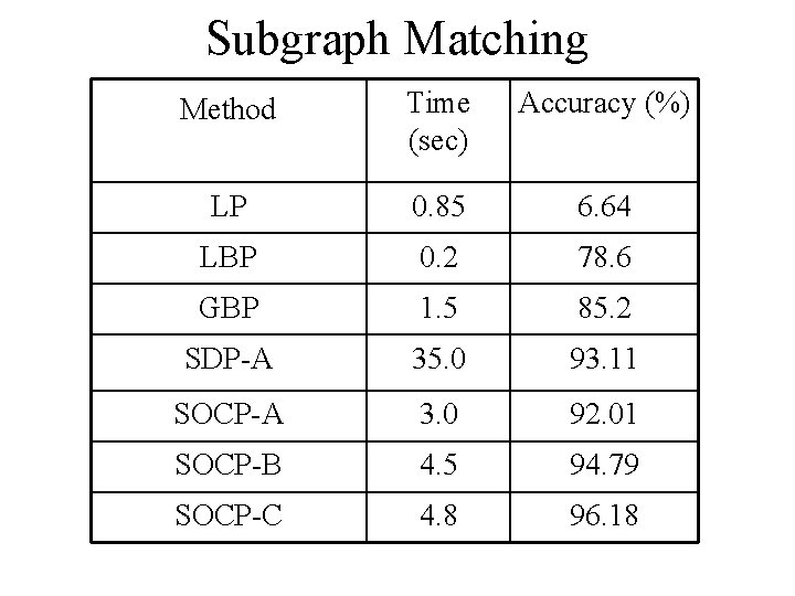
Subgraph Matching Method Time (sec) Accuracy (%) LP 0. 85 6. 64 LBP 0. 2 78. 6 GBP 1. 5 85. 2 SDP-A 35. 0 93. 11 SOCP-A 3. 0 92. 01 SOCP-B 4. 5 94. 79 SOCP-C 4. 8 96. 18

Outline • Integer Programming Formulation • Previous Work • Our Approach – Second Order Cone Programming (SOCP) – SOCP Relaxation – Robust Truncated Model • Applications – Subgraph Matching – Pictorial Structures

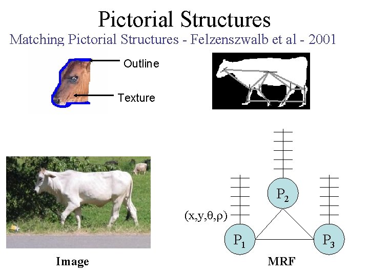
Pictorial Structures Matching Pictorial Structures - Felzenszwalb et al - 2001 Outline Texture P 2 (x, y, , ) P 1 Image P 3 MRF

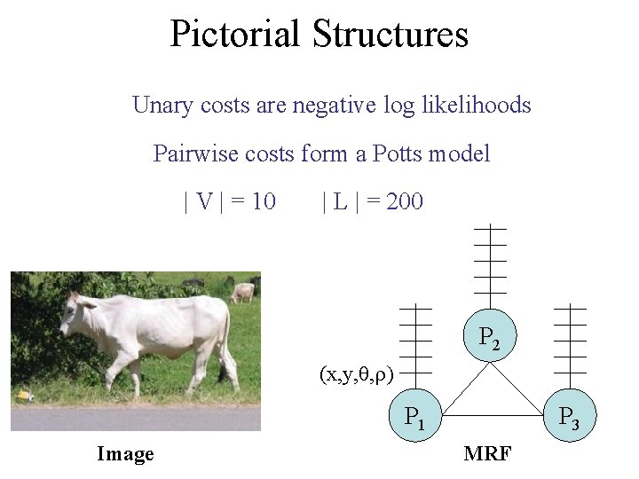
Pictorial Structures Unary costs are negative log likelihoods Pairwise costs form a Potts model | V | = 10 | L | = 200 P 2 (x, y, , ) P 1 Image P 3 MRF

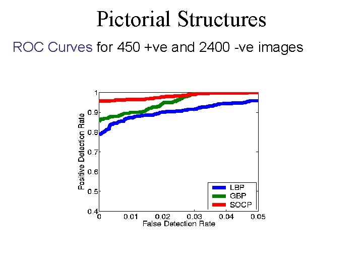
Pictorial Structures ROC Curves for 450 +ve and 2400 -ve images

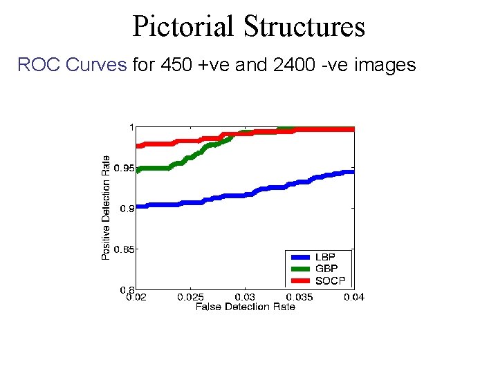
Pictorial Structures ROC Curves for 450 +ve and 2400 -ve images

Conclusions • We presented an SOCP relaxation to solve MRF • More efficient than SDP • More accurate than LP, LBP, GBP • #variables can be reduced for Robust Truncated Model • Provides excellent results for subgraph matching and pictorial structures

Future Work • Quality of solution – Additive bounds exist – Multiplicative bounds for special cases ? ? – What are good C’s. • Message passing algorithm ? ? – Similar to TRW-S or -expansion – To handle image sized MRF