A Revealing Introduction to Hidden Markov Models Mark

A Revealing Introduction to Hidden Markov Models Mark Stamp A Revealing Introduction to HMMs 1

Hidden Markov Models q What is a hidden Markov model (HMM)? o A machine learning technique… o …trained via a discrete hill climb technique o Two for the price of one! q Where are HMMs used? o Speech recognition, information security, and far too many other things to list o Q: Why are HMMs so useful? o A: Widely applicable and efficient algorithms A Revealing Introduction to HMMs 2

Markov Chain q Markov chain o “Memoryless random process” o Transitions depend only on current state (Markov chain of order 1)… o …and transition probability matrix q Example? o See next slide… A Revealing Introduction to HMMs 3

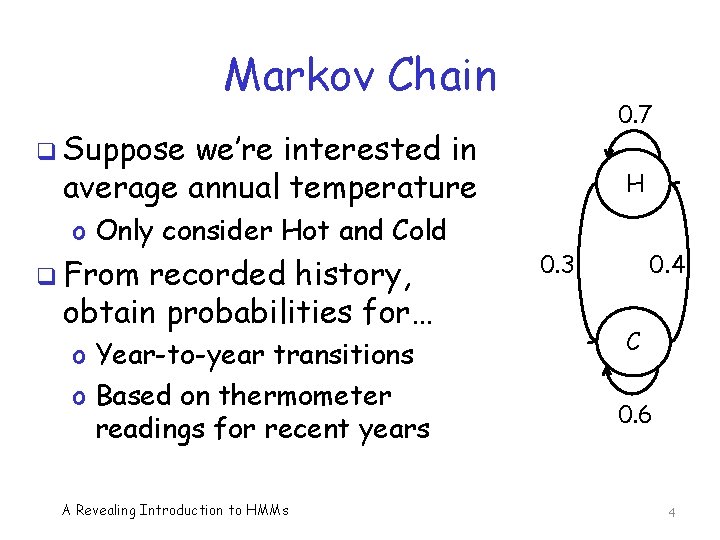
Markov Chain 0. 7 q Suppose we’re interested in average annual temperature o Only consider Hot and Cold q From recorded history, obtain probabilities for… o Year-to-year transitions o Based on thermometer readings for recent years A Revealing Introduction to HMMs H 0. 3 0. 4 C 0. 6 4

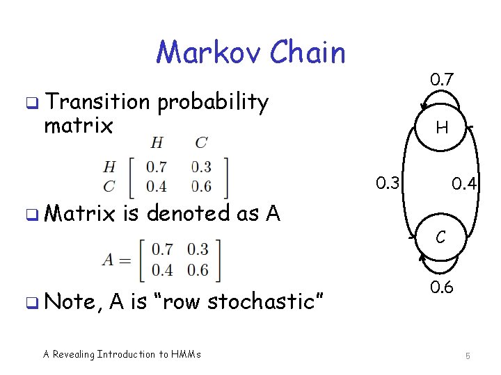
Markov Chain q Transition matrix 0. 7 probability H 0. 3 q Matrix q Note, is denoted as A A is “row stochastic” A Revealing Introduction to HMMs 0. 4 C 0. 6 5

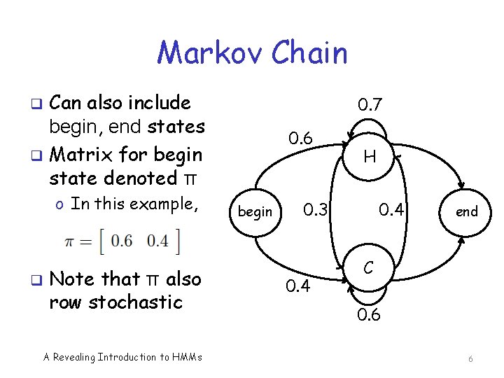
Markov Chain Can also include begin, end states q Matrix for begin state denoted π 0. 7 q o In this example, q Note that π also row stochastic A Revealing Introduction to HMMs 0. 6 begin H 0. 3 0. 4 end C 0. 6 6

Hidden Markov Model q HMM includes a Markov chain o But the Markov process is “hidden”, i. e. , we can’t directly observe the Markov process o Instead, observe things that are probabilistically related to hidden states o It’s as if there is a “curtain” between Markov chain and the observations q Example on next few slides… A Revealing Introduction to HMMs 7

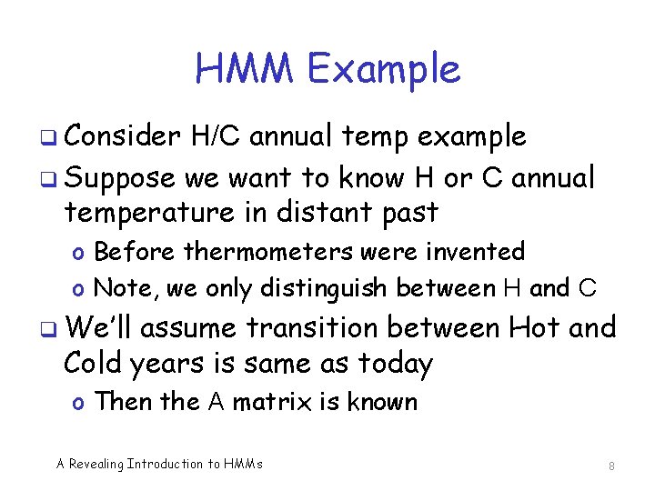
HMM Example q Consider H/C annual temp example q Suppose we want to know H or C annual temperature in distant past o Before thermometers were invented o Note, we only distinguish between H and C q We’ll assume transition between Hot and Cold years is same as today o Then the A matrix is known A Revealing Introduction to HMMs 8

HMM Example q Assume temps follow a Markov process o But, we cannot observe temperature in past q We find modern evidence that tree ring size is related to temperature o Discover this by looking at recent data q We only consider 3 tree ring sizes o Small, Medium, Large (S, M, L, respectively) q Measure tree ring sizes and recorded temperatures to determine relationship A Revealing Introduction to HMMs 9

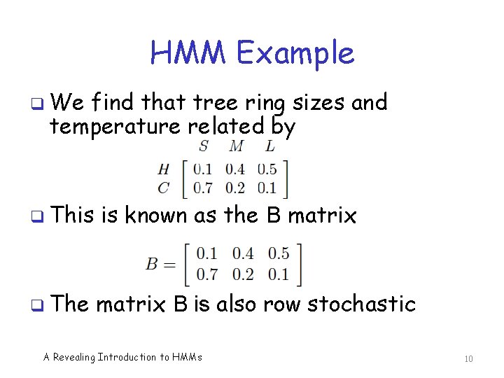
HMM Example q We find that tree ring sizes and temperature related by q This is known as the B matrix q The matrix B is also row stochastic A Revealing Introduction to HMMs 10

HMM Example q Can we now find H/C temps in past? q We cannot measure (observe) temps q But we can measure tree ring sizes… q …and tree ring sizes related to temps o By the probabilities in the B matrix q Can we say something intelligent about temps over some interval in the past? A Revealing Introduction to HMMs 11

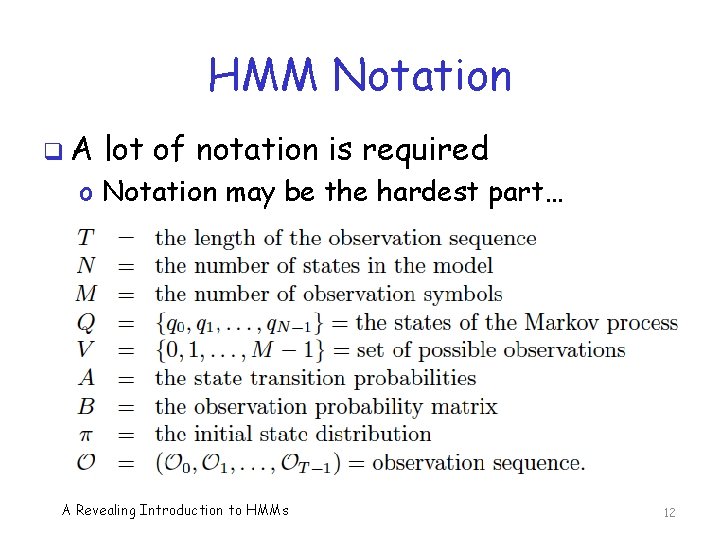
HMM Notation q. A lot of notation is required o Notation may be the hardest part… A Revealing Introduction to HMMs 12

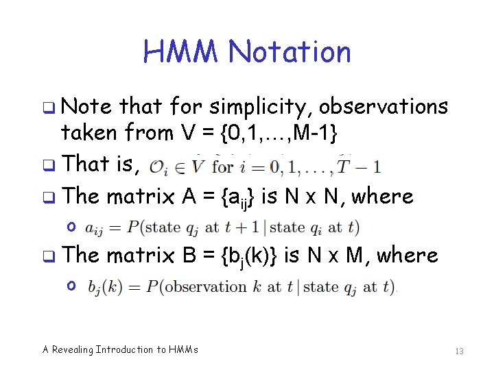
HMM Notation q Note that for simplicity, observations taken from V = {0, 1, …, M-1} q That is, q The matrix A = {aij} is N x N, where o q The o matrix B = {bj(k)} is N x M, where A Revealing Introduction to HMMs 13

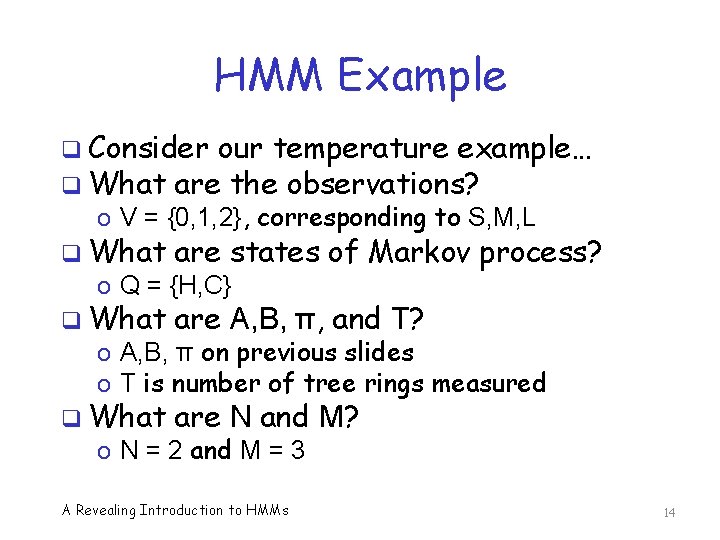
HMM Example q Consider our temperature example… q What are the observations? o V = {0, 1, 2}, corresponding to S, M, L q What are states of Markov process? o Q = {H, C} q What are A, B, π, and T? q What are N and M? o A, B, π on previous slides o T is number of tree rings measured o N = 2 and M = 3 A Revealing Introduction to HMMs 14

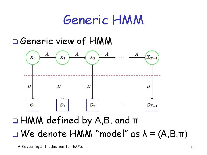
Generic HMM q Generic view of HMM q HMM defined by A, B, and π q We denote HMM “model” as λ = (A, B, π) A Revealing Introduction to HMMs 15

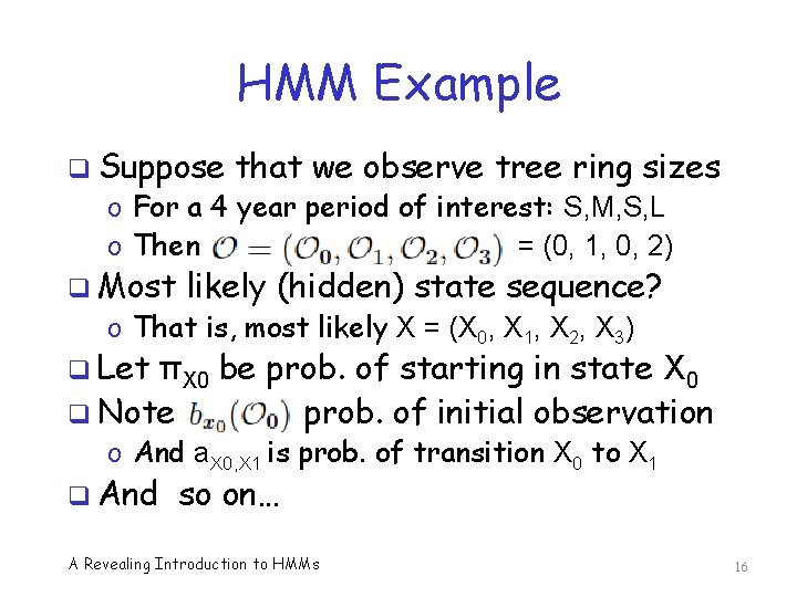
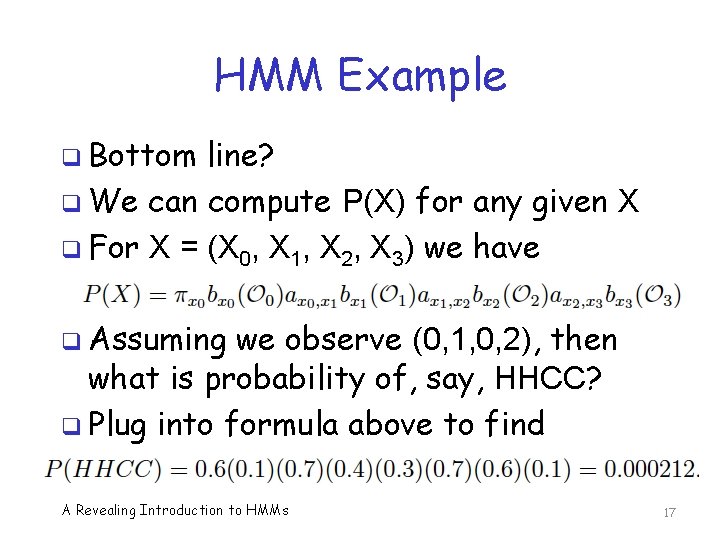
HMM Example q Suppose that we observe tree ring sizes o For a 4 year period of interest: S, M, S, L o Then = (0, 1, 0, 2) q Most likely (hidden) state sequence? o That is, most likely X = (X 0, X 1, X 2, X 3) q Let πX 0 be prob. of starting in state X 0 q Note prob. of initial observation o And a. X 0, X 1 is prob. of transition X 0 to X 1 q And so on… A Revealing Introduction to HMMs 16

HMM Example q Bottom line? q We can compute P(X) for any given X q For X = (X 0, X 1, X 2, X 3) we have q Assuming we observe (0, 1, 0, 2), then what is probability of, say, HHCC? q Plug into formula above to find A Revealing Introduction to HMMs 17

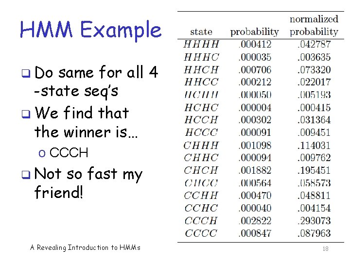
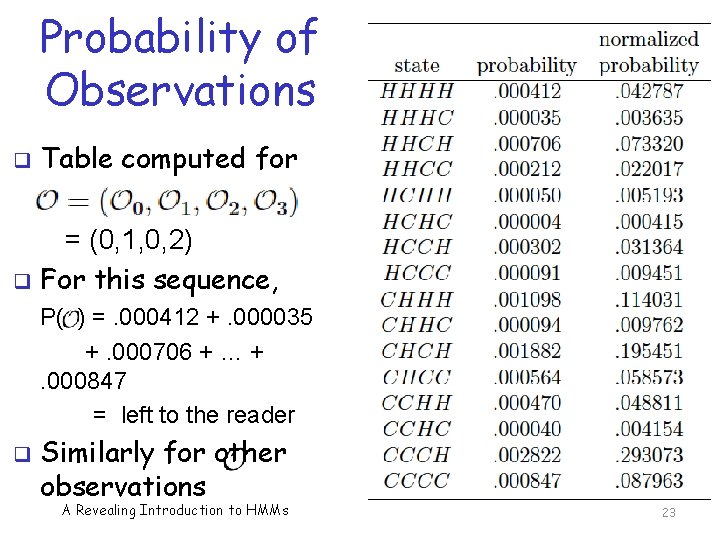
HMM Example q Do same for all 4 -state seq’s q We find that the winner is… o CCCH q Not so fast my friend! A Revealing Introduction to HMMs 18

HMM Example q The path CCCH scores the highest q In dynamic programming (DP), we find highest scoring path q But, in HMM we maximize expected number of correct states o Sometimes called “EM algorithm” o For “expectation maximization” q How does HMM work in this example? A Revealing Introduction to HMMs 19

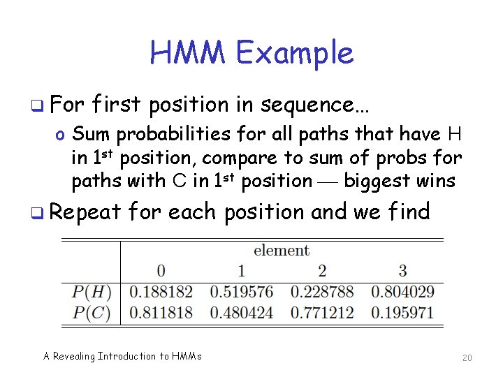
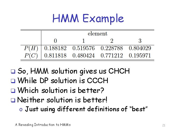
HMM Example q For first position in sequence… o Sum probabilities for all paths that have H in 1 st position, compare to sum of probs for paths with C in 1 st position biggest wins q Repeat for each position and we find A Revealing Introduction to HMMs 20

HMM Example q So, HMM solution gives us CHCH q While DP solution is CCCH q Which solution is better? q Neither solution is better! o Just using different definitions of “best” A Revealing Introduction to HMMs 21

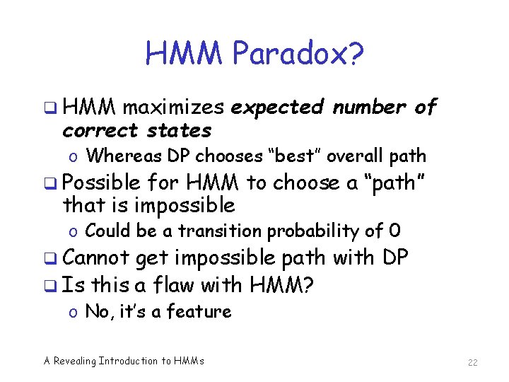
HMM Paradox? q HMM maximizes expected number of correct states o Whereas DP chooses “best” overall path q Possible for HMM to choose a “path” that is impossible o Could be a transition probability of 0 q Cannot get impossible path with DP q Is this a flaw with HMM? o No, it’s a feature A Revealing Introduction to HMMs 22

Probability of Observations q Table computed for = (0, 1, 0, 2) q For this sequence, P( ) =. 000412 +. 000035 +. 000706 + … +. 000847 = left to the reader q Similarly for other observations A Revealing Introduction to HMMs 23

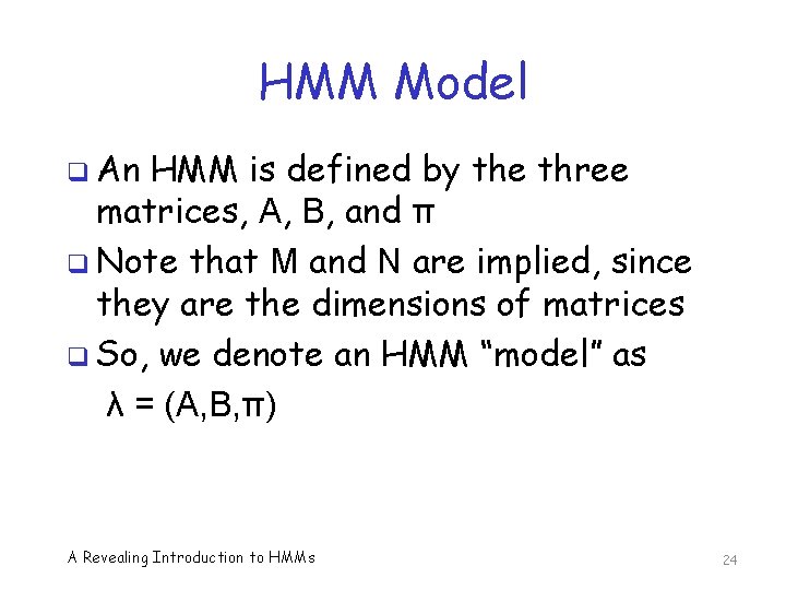
HMM Model q An HMM is defined by the three matrices, A, B, and π q Note that M and N are implied, since they are the dimensions of matrices q So, we denote an HMM “model” as λ = (A, B, π) A Revealing Introduction to HMMs 24

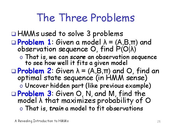
The Three Problems q HMMs used to solve 3 problems q Problem 1: Given a model λ = (A, B, π) and observation sequence O, find P(O|λ) o That is, we can score an observation sequence to see how well it fits a given model q Problem 2: Given λ = (A, B, π) and O, find an optimal state sequence (in HMM sense) o Uncover hidden part (like previous example) q Problem 3: Given O, N, and M, find the model λ that maximizes probability of O o That is, train a model to fit observations A Revealing Introduction to HMMs 25

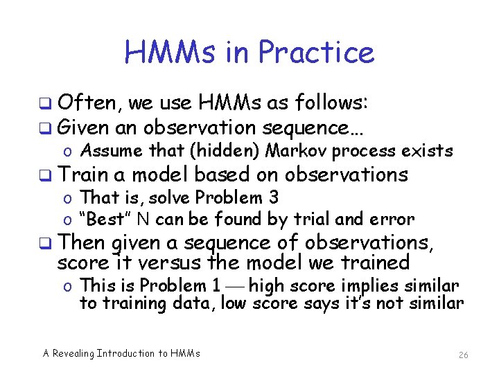
HMMs in Practice q Often, we use HMMs as follows: q Given an observation sequence… o Assume that (hidden) Markov process exists q Train a model based on observations o That is, solve Problem 3 o “Best” N can be found by trial and error q Then given a sequence of observations, score it versus the model we trained o This is Problem 1 high score implies similar to training data, low score says it’s not similar A Revealing Introduction to HMMs 26

HMMs in Practice q Previous slide gives sense in which HMM is a “machine learning” technique o To train model, we do not need to specify anything except the parameter N o “Best” N often found by trial and error q So, we don’t need to think too much o Just train HMM and then use it o Practical, since efficient algorithms for training HMM and scoring A Revealing Introduction to HMMs 27

The Three Solutions q We give detailed solutions to 3 problems o Note: We must find efficient solutions q The three problems: o Problem 1: Score an observation sequence versus a given model o Problem 2: Given a model, “uncover” hidden part o Problem 3: Given an observation sequence, train a model q Recall that we considered example for 2 and 1 o But direct solutions are soooooo… inefficient A Revealing Introduction to HMMs 28

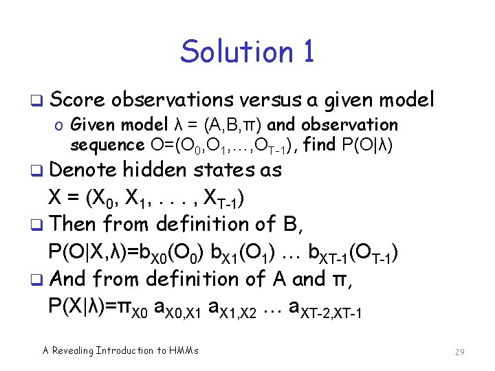
Solution 1 q Score observations versus a given model o Given model λ = (A, B, π) and observation sequence O=(O 0, O 1, …, OT-1), find P(O|λ) q Denote hidden states as X = (X 0, X 1, . . . , XT-1) q Then from definition of B, P(O|X, λ)=b. X 0(O 0) b. X 1(O 1) … b. XT-1(OT-1) q And from definition of A and π, P(X|λ)=πX 0 a. X 0, X 1 a. X 1, X 2 … a. XT-2, XT-1 A Revealing Introduction to HMMs 29

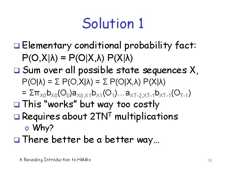
Solution 1 q Elementary conditional probability fact: P(O, X|λ) = P(O|X, λ) P(X|λ) q Sum over all possible state sequences X, P(O|λ) = Σ P(O, X|λ) = Σ P(O|X, λ) P(X|λ) = ΣπX 0 b. X 0(O 0)a. X 0, X 1 b. X 1(O 1)…a. XT-2, XT-1 b. XT-1(OT-1) q This “works” but way too costly q Requires about 2 TNT multiplications o Why? q There better be a better way… A Revealing Introduction to HMMs 30

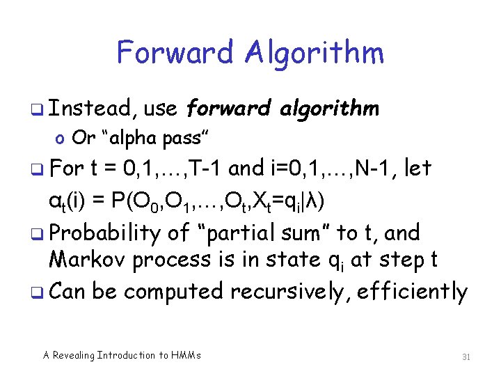
Forward Algorithm q Instead, use forward algorithm o Or “alpha pass” q For t = 0, 1, …, T-1 and i=0, 1, …, N-1, let αt(i) = P(O 0, O 1, …, Ot, Xt=qi|λ) q Probability of “partial sum” to t, and Markov process is in state qi at step t q Can be computed recursively, efficiently A Revealing Introduction to HMMs 31

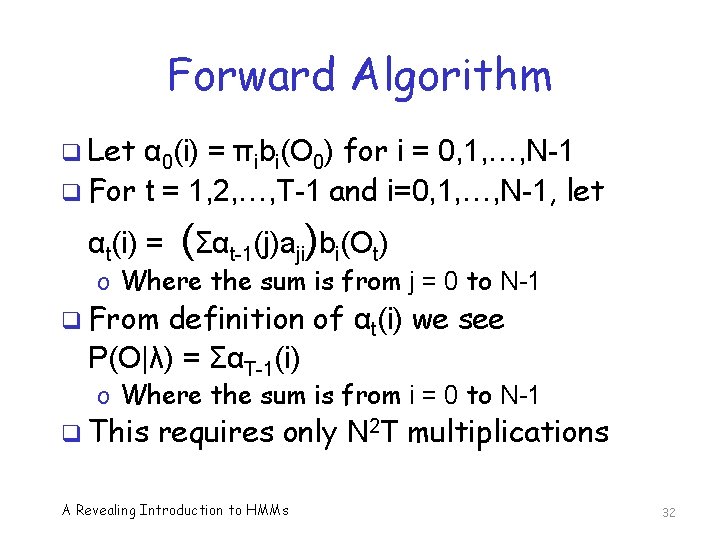
Forward Algorithm q Let α 0(i) = πibi(O 0) for i = 0, 1, …, N-1 q For t = 1, 2, …, T-1 and i=0, 1, …, N-1, let αt(i) = (Σαt-1(j)aji)bi(Ot) o Where the sum is from j = 0 to N-1 q From definition of αt(i) we see P(O|λ) = ΣαT-1(i) o Where the sum is from i = 0 to N-1 q This requires only N 2 T multiplications A Revealing Introduction to HMMs 32

Solution 2 q Given a model, find hidden states o Given λ = (A, B, π) and O, find an optimal state sequence o Recall that optimal means “maximize expected number of correct states” o In contrast, DP finds best scoring path q For temp/tree ring example, solved this o But hopelessly inefficient approach q. A better way: backward algorithm o Or “beta pass” A Revealing Introduction to HMMs 33

Backward Algorithm q For t = 0, 1, …, T-1 and i = 0, 1, …, N-1, let βt(i) = P(Ot+1, Ot+2, …, OT-1|Xt=qi, λ) q Probability of partial sum from t to end and Markov process in state qi at step t q Analogous to the forward algorithm q As with forward algorithm, this can be computed recursively and efficiently A Revealing Introduction to HMMs 34

Backward Algorithm q Let βT-1(i) = 1 for i = 0, 1, …, N-1 q For t = T-2, T-3, …, 1 and i = 0, 1, …, N-1, let βt(i) = Σaijbj(Ot+1)βt+1(j) q Where the sum is from j = 0 to N-1 A Revealing Introduction to HMMs 35

Solution 2 q For t = 1, 2, …, T-1 and i=0, 1, …, N-1 define γt(i) = P(Xt=qi|O, λ) o Most likely state at t is qi that maximizes γt(i) q Note that γt(i) = αt(i)βt(i)/P(O|λ) o And recall P(O|λ) = ΣαT-1(i) q The bottom line? o Forward algorithm solves Problem 1 o Forward/backward algorithms solve Problem 2 (how? ) A Revealing Introduction to HMMs 36

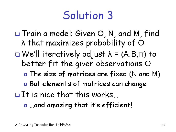
Solution 3 q Train a model: Given O, N, and M, find λ that maximizes probability of O q We’ll iteratively adjust λ = (A, B, π) to better fit the given observations O o The size of matrices are fixed (N and M) o But elements of matrices can change q It is nice that this works… o …and amazing that it’s efficient! A Revealing Introduction to HMMs 37

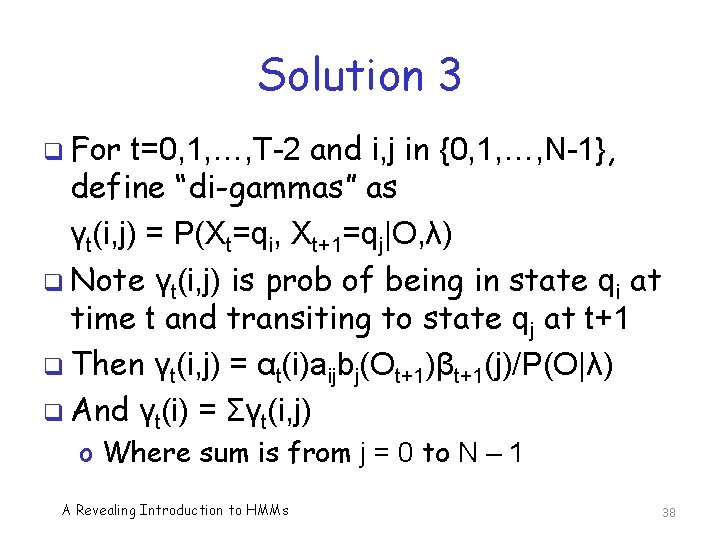
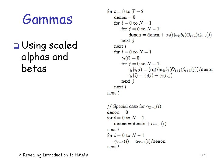
Solution 3 q For t=0, 1, …, T-2 and i, j in {0, 1, …, N-1}, define “di-gammas” as γt(i, j) = P(Xt=qi, Xt+1=qj|O, λ) q Note γt(i, j) is prob of being in state qi at time t and transiting to state qj at t+1 q Then γt(i, j) = αt(i)aijbj(Ot+1)βt+1(j)/P(O|λ) q And γt(i) = Σγt(i, j) o Where sum is from j = 0 to N – 1 A Revealing Introduction to HMMs 38

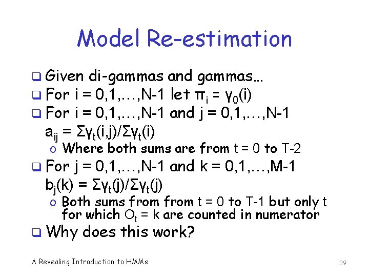
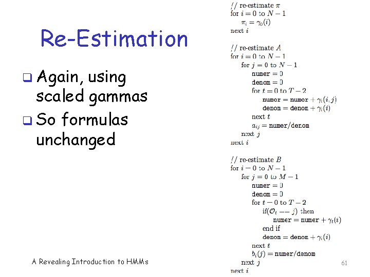
Model Re-estimation q Given di-gammas and gammas… q For i = 0, 1, …, N-1 let πi = γ 0(i) q For i = 0, 1, …, N-1 and j = 0, 1, …, N-1 aij = Σγt(i, j)/Σγt(i) o Where both sums are from t = 0 to T-2 q For j = 0, 1, …, N-1 and k = 0, 1, …, M-1 bj(k) = Σγt(j)/Σγt(j) o Both sums from t = 0 to T-1 but only t for which Ot = k are counted in numerator q Why does this work? A Revealing Introduction to HMMs 39

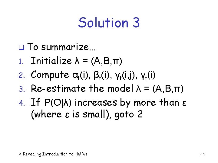
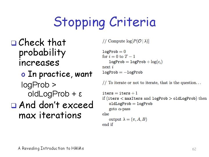
Solution 3 q To 1. 2. 3. 4. summarize… Initialize λ = (A, B, π) Compute αt(i), βt(i), γt(i, j), γt(i) Re-estimate the model λ = (A, B, π) If P(O|λ) increases by more than ε (where ε is small), goto 2 A Revealing Introduction to HMMs 40

Solution 3 q Some fine points… q Model initialization o If we have a good guess for λ = (A, B, π) then we can use it for initialization o If not, let πi ≈ 1/N, ai, j ≈ 1/N, bj(k) ≈ 1/M o Subject to row stochastic conditions o But, do not initialize to exactly uniform values q Stopping conditions o Stop after some number of iterations and/or… o Stop if increase in P(O|λ) is too small A Revealing Introduction to HMMs 41

HMM as Discrete Hill Climb q Algorithm on previous slides shows that HMM is a “discrete hill climb” q HMM consists of discrete states, Xt o “Climb” on the elements of the matrices q And re-estimation process improves model by modifying parameters o So, “climbs” toward improved model o This happens in a high-dimensional space A Revealing Introduction to HMMs 42

Dynamic Programming q Brief detour… q For λ = (A, B, π) as above, it’s easy to define a dynamic program (DP) q Executive summary: o DP is forward algorithm, with “sum” replaced by “max” q Details on next few slides A Revealing Introduction to HMMs 43

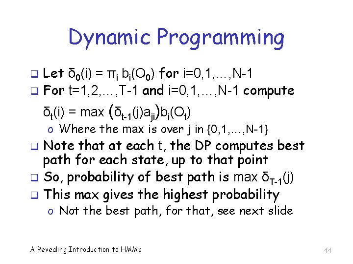
Dynamic Programming q q Let δ 0(i) = πi bi(O 0) for i=0, 1, …, N-1 For t=1, 2, …, T-1 and i=0, 1, …, N-1 compute δt(i) = max (δt-1(j)aji)bi(Ot) o Where the max is over j in {0, 1, …, N-1} q q q Note that at each t, the DP computes best path for each state, up to that point So, probability of best path is max δT-1(j) This max gives the highest probability o Not the best path, for that, see next slide A Revealing Introduction to HMMs 44

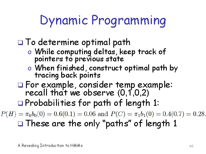
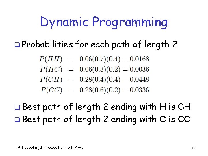
Dynamic Programming q To determine optimal path o While computing deltas, keep track of pointers to previous state o When finished, construct optimal path by tracing back points q For example, consider temp example: recall that we observe (0, 1, 0, 2) q Probabilities for path of length 1: q These are the only “paths” of length 1 A Revealing Introduction to HMMs 45

Dynamic Programming q Probabilities for each path of length 2 q Best path of length 2 ending with H is CH q Best path of length 2 ending with C is CC A Revealing Introduction to HMMs 46

Dynamic Program q Continuing, we compute best path ending at H and C at each step q And save pointers why? A Revealing Introduction to HMMs 47

Dynamic Program q Best final score is. 002822 o And thanks to pointers, best path is CCCH q But what about underflow? o A serious problem in bigger cases A Revealing Introduction to HMMs 48

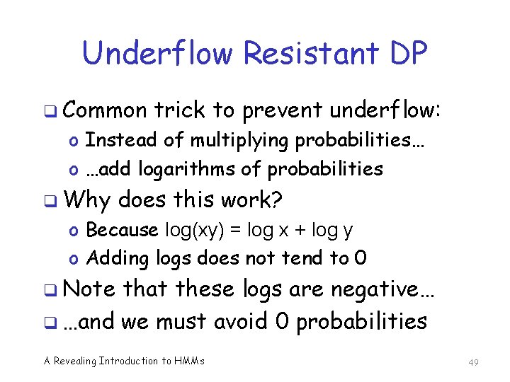
Underflow Resistant DP q Common trick to prevent underflow: o Instead of multiplying probabilities… o …add logarithms of probabilities q Why does this work? o Because log(xy) = log x + log y o Adding logs does not tend to 0 q Note that these logs are negative… q …and we must avoid 0 probabilities A Revealing Introduction to HMMs 49

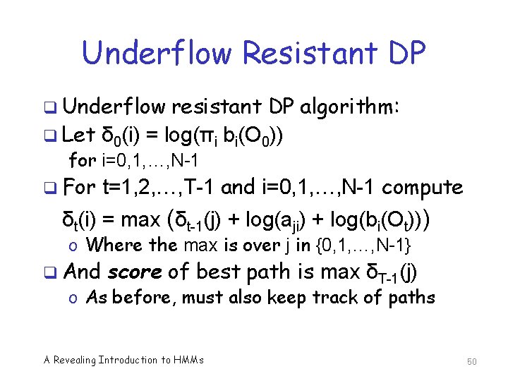
Underflow Resistant DP q Underflow resistant DP algorithm: q Let δ 0(i) = log(πi bi(O 0)) for i=0, 1, …, N-1 q For t=1, 2, …, T-1 and i=0, 1, …, N-1 compute δt(i) = max (δt-1(j) + log(aji) + log(bi(Ot))) o Where the max is over j in {0, 1, …, N-1} q And score of best path is max δT-1(j) o As before, must also keep track of paths A Revealing Introduction to HMMs 50

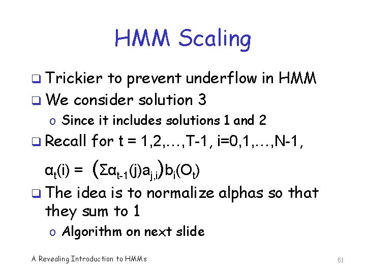
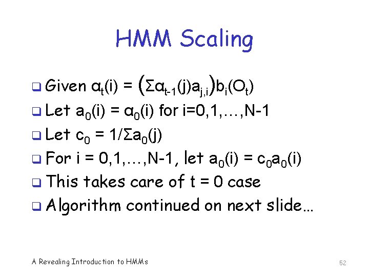
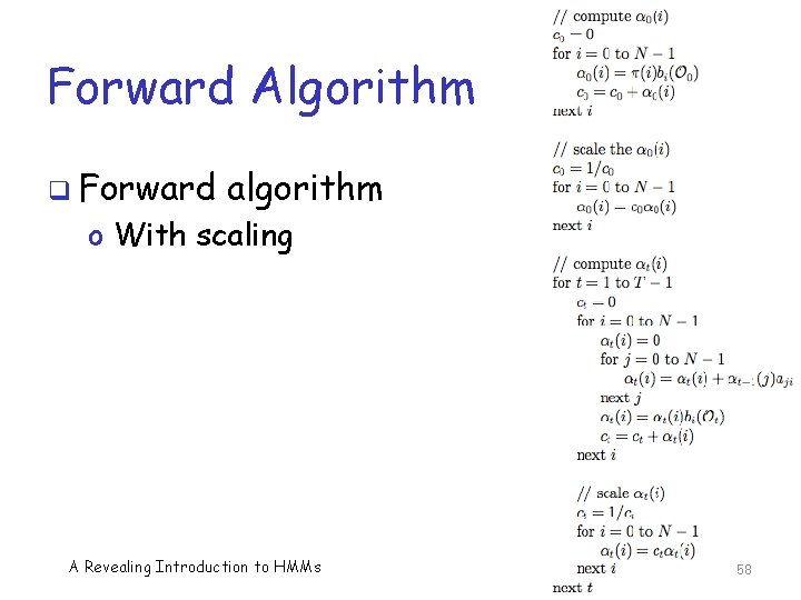
HMM Scaling q Trickier to prevent underflow in HMM q We consider solution 3 o Since it includes solutions 1 and 2 q Recall αt(i) = for t = 1, 2, …, T-1, i=0, 1, …, N-1, (Σαt-1(j)aj, i)bi(Ot) q The idea is to normalize alphas so that they sum to 1 o Algorithm on next slide A Revealing Introduction to HMMs 51

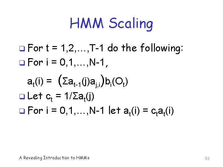
HMM Scaling q Given αt(i) = (Σαt-1(j)aj, i)bi(Ot) q Let a 0(i) = α 0(i) for i=0, 1, …, N-1 q Let c 0 = 1/Σa 0(j) q For i = 0, 1, …, N-1, let a 0(i) = c 0 a 0(i) q This takes care of t = 0 case q Algorithm continued on next slide… A Revealing Introduction to HMMs 52

HMM Scaling q For t = 1, 2, …, T-1 do the following: q For i = 0, 1, …, N-1, at(i) = (Σat-1(j)aj, i)bi(Ot) q Let ct = 1/Σat(j) q For i = 0, 1, …, N-1 let at(i) = ctat(i) A Revealing Introduction to HMMs 53

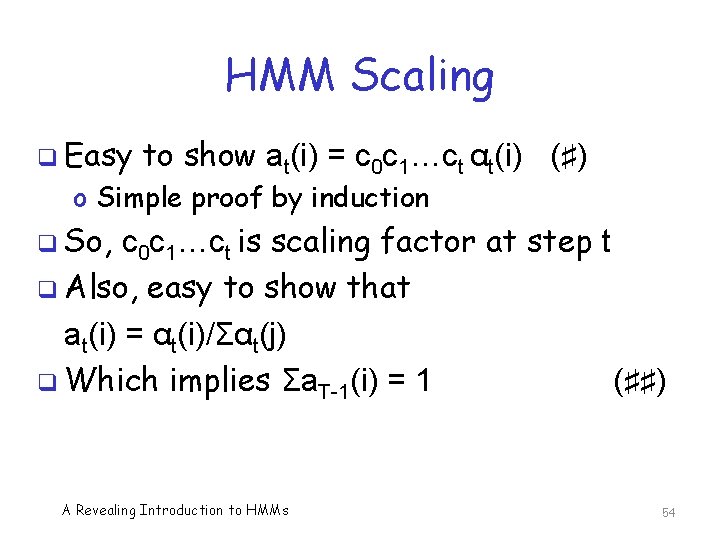
HMM Scaling q Easy to show at(i) = c 0 c 1…ct αt(i) (♯) o Simple proof by induction q So, c 0 c 1…ct is scaling factor at step t q Also, easy to show that at(i) = αt(i)/Σαt(j) q Which implies Σa. T-1(i) = 1 (♯♯) A Revealing Introduction to HMMs 54

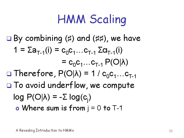
HMM Scaling q By combining (♯) and (♯♯), we have 1 = Σa. T-1(i) = c 0 c 1…c. T-1 ΣαT-1(i) = c 0 c 1…c. T-1 P(O|λ) q Therefore, P(O|λ) = 1 / c 0 c 1…c. T-1 q To avoid underflow, we compute log P(O|λ) = -Σ log(cj) o Where sum is from j = 0 to T-1 A Revealing Introduction to HMMs 55

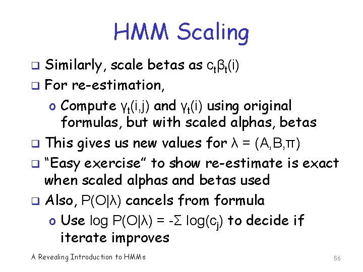
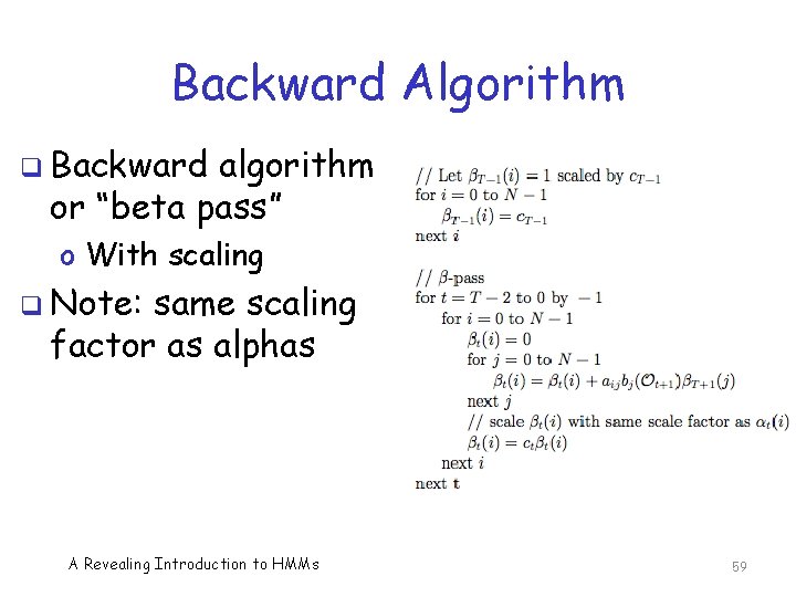
HMM Scaling Similarly, scale betas as ctβt(i) q For re-estimation, o Compute γt(i, j) and γt(i) using original formulas, but with scaled alphas, betas q This gives us new values for λ = (A, B, π) q “Easy exercise” to show re-estimate is exact when scaled alphas and betas used q Also, P(O|λ) cancels from formula o Use log P(O|λ) = -Σ log(cj) to decide if iterate improves q A Revealing Introduction to HMMs 56

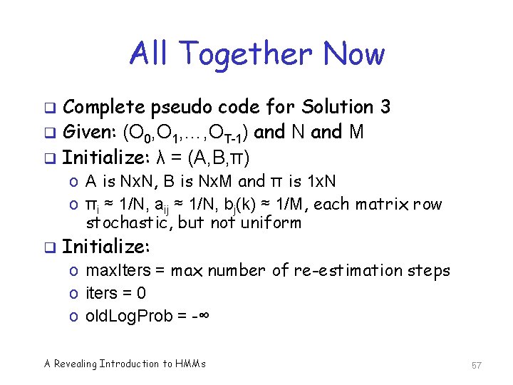
All Together Now q q q Complete pseudo code for Solution 3 Given: (O 0, O 1, …, OT-1) and N and M Initialize: λ = (A, B, π) o A is Nx. N, B is Nx. M and π is 1 x. N o πi ≈ 1/N, aij ≈ 1/N, bj(k) ≈ 1/M, each matrix row stochastic, but not uniform q Initialize: o max. Iters = max number of re-estimation steps o iters = 0 o old. Log. Prob = -∞ A Revealing Introduction to HMMs 57

Forward Algorithm q Forward algorithm o With scaling A Revealing Introduction to HMMs 58

Backward Algorithm q Backward algorithm or “beta pass” o With scaling q Note: same scaling factor as alphas A Revealing Introduction to HMMs 59

Gammas q Using scaled alphas and betas A Revealing Introduction to HMMs 60

Re-Estimation q Again, using scaled gammas q So formulas unchanged A Revealing Introduction to HMMs 61

Stopping Criteria q Check that probability increases o In practice, want log. Prob > old. Log. Prob + ε q And don’t exceed max iterations A Revealing Introduction to HMMs 62

References q M. Stamp, A revealing introduction to hidden Markov models q L. R. Rabiner, A tutorial on hidden Markov models and selected applications in speech recognition q R. L. Cave & L. P. Neuwirth, Hidden Markov models for English A Revealing Introduction to HMMs 63