Chapter 4 The Simplex Algorithm and Goal Programming

Chapter 4 The Simplex Algorithm and Goal Programming to accompany Operations Research: Applications and Algorithms 4 th edition by Wayne L. Winston Copyright (c) 2004 Brooks/Cole, a division of Thomson Learning, Inc.

4. 1 How to Convert an LP to Standard Form n Before the simplex algorithm can be used to solve an LP, the LP must be converted into a problem where all the constraints are equations and all variables are nonnegative. n An LP in this form is said to be in standard form. 2

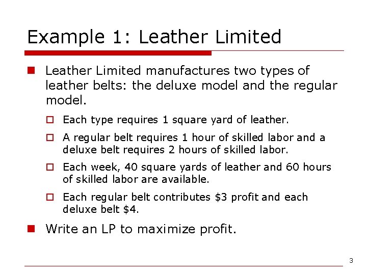
Example 1: Leather Limited n Leather Limited manufactures two types of leather belts: the deluxe model and the regular model. o Each type requires 1 square yard of leather. o A regular belt requires 1 hour of skilled labor and a deluxe belt requires 2 hours of skilled labor. o Each week, 40 square yards of leather and 60 hours of skilled labor are available. o Each regular belt contributes $3 profit and each deluxe belt $4. n Write an LP to maximize profit. 3

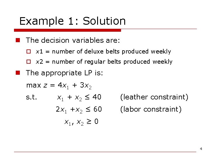
Example 1: Solution n The decision variables are: o x 1 = number of deluxe belts produced weekly o x 2 = number of regular belts produced weekly n The appropriate LP is: max z = 4 x 1 + 3 x 2 s. t. x 1 + x 2 ≤ 40 (leather constraint) 2 x 1 +x 2 ≤ 60 (labor constraint) x 1, x 2 ≥ 0 4

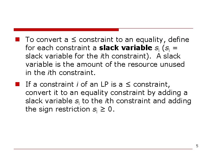
n To convert a ≤ constraint to an equality, define for each constraint a slack variable si (si = slack variable for the ith constraint). A slack variable is the amount of the resource unused in the ith constraint. n If a constraint i of an LP is a ≤ constraint, convert it to an equality constraint by adding a slack variable si to the ith constraint and adding the sign restriction si ≥ 0. 5

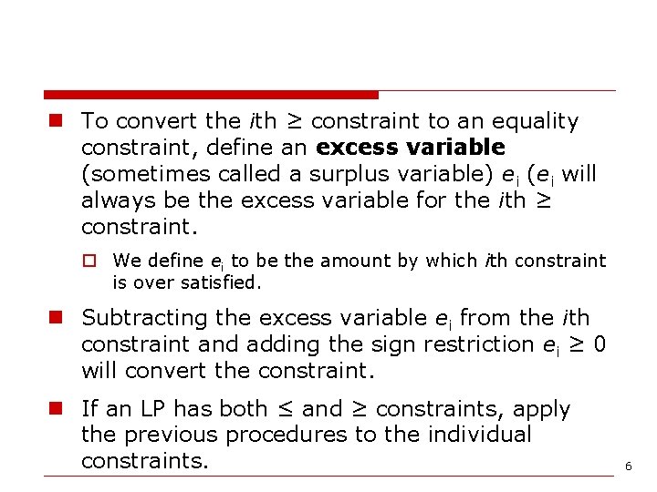
n To convert the ith ≥ constraint to an equality constraint, define an excess variable (sometimes called a surplus variable) ei (ei will always be the excess variable for the ith ≥ constraint. o We define ei to be the amount by which ith constraint is over satisfied. n Subtracting the excess variable ei from the ith constraint and adding the sign restriction ei ≥ 0 will convert the constraint. n If an LP has both ≤ and ≥ constraints, apply the previous procedures to the individual constraints. 6

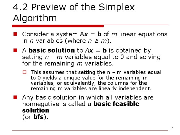
4. 2 Preview of the Simplex Algorithm n Consider a system Ax = b of m linear equations in n variables (where n ≥ m). n A basic solution to Ax = b is obtained by setting n – m variables equal to 0 and solving for the remaining m variables. o This assumes that setting the n – m variables equal to 0 yields a unique value for the remaining m variables, or equivalently, the columns for the remaining m variables are linearly independent. n Any basic solution in which all variables are nonnegative is called a basic feasible solution (or bfs). 7

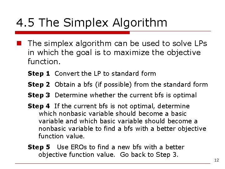
4. 5 The Simplex Algorithm n The simplex algorithm can be used to solve LPs in which the goal is to maximize the objective function. Step 1 Convert the LP to standard form Step 2 Obtain a bfs (if possible) from the standard form Step 3 Determine whether the current bfs is optimal Step 4 If the current bfs is not optimal, determine which nonbasic variable should become a basic variable and which basic variable should become a nonbasic variable to find a bfs with a better objective function value. Step 5 Use EROs to find a new bfs with a better objective function value. Go back to Step 3. 12

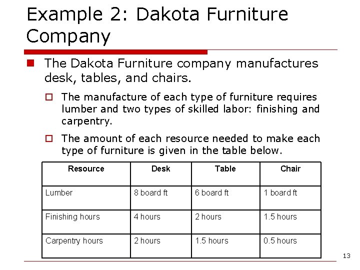
Example 2: Dakota Furniture Company n The Dakota Furniture company manufactures desk, tables, and chairs. o The manufacture of each type of furniture requires lumber and two types of skilled labor: finishing and carpentry. o The amount of each resource needed to make each type of furniture is given in the table below. Resource Desk Table Chair Lumber 8 board ft 6 board ft 1 board ft Finishing hours 4 hours 2 hours 1. 5 hours Carpentry hours 2 hours 1. 5 hours 0. 5 hours 13

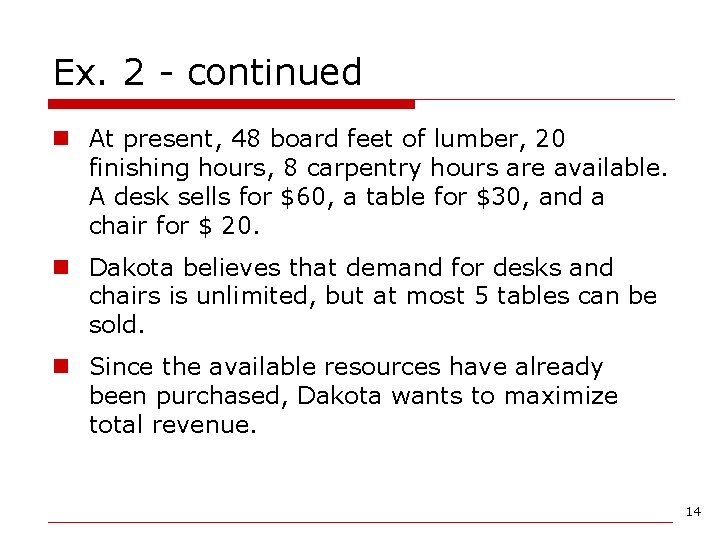
Ex. 2 - continued n At present, 48 board feet of lumber, 20 finishing hours, 8 carpentry hours are available. A desk sells for $60, a table for $30, and a chair for $ 20. n Dakota believes that demand for desks and chairs is unlimited, but at most 5 tables can be sold. n Since the available resources have already been purchased, Dakota wants to maximize total revenue. 14

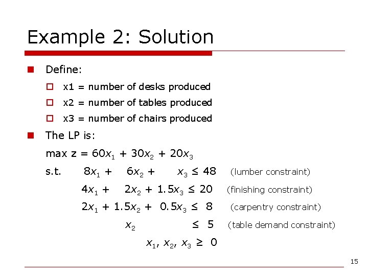
Example 2: Solution n Define: o x 1 = number of desks produced o x 2 = number of tables produced o x 3 = number of chairs produced n The LP is: max z = 60 x 1 + 30 x 2 + 20 x 3 s. t. 8 x 1 + 6 x 2 + x 3 ≤ 48 4 x 1 + 2 x 2 + 1. 5 x 3 ≤ 20 2 x 1 + 1. 5 x 2 + 0. 5 x 3 ≤ 8 x 2 ≤ 5 (lumber constraint) (finishing constraint) (carpentry constraint) (table demand constraint) x 1, x 2, x 3 ≥ 0 15

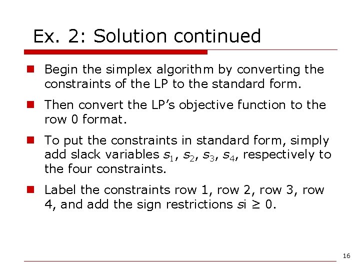
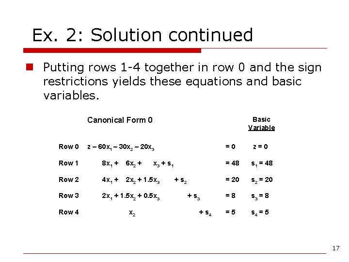
Ex. 2: Solution continued n Begin the simplex algorithm by converting the constraints of the LP to the standard form. n Then convert the LP’s objective function to the row 0 format. n To put the constraints in standard form, simply add slack variables s 1, s 2, s 3, s 4, respectively to the four constraints. n Label the constraints row 1, row 2, row 3, row 4, and add the sign restrictions si ≥ 0. 16

Ex. 2: Solution continued n Putting rows 1 -4 together in row 0 and the sign restrictions yields these equations and basic variables. Basic Variable Canonical Form 0 Row 0 z – 60 x 1 – 30 x 2 – 20 x 3 Row 1 8 x 1 + 6 x 2 + x 3 + s 1 Row 2 4 x 1 + 2 x 2 + 1. 5 x 3 Row 3 2 x 1 + 1. 5 x 2 + 0. 5 x 3 Row 4 x 2 + s 3 + s 4 =0 z=0 = 48 s 1 = 48 = 20 s 2 = 20 =8 s 3 = 8 =5 s 4 = 5 17

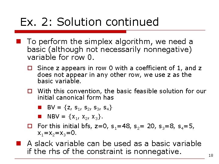
Ex. 2: Solution continued n To perform the simplex algorithm, we need a basic (although not necessarily nonnegative) variable for row 0. o Since z appears in row 0 with a coefficient of 1, and z does not appear in any other row, we use z as the basic variable. o With this convention, the basic feasible solution for our initial canonical form has n BV = {z, s 1, s 2, s 3, s 4} n NBV = {x 1, x 2, x 3}. o For this initial bfs, z=0, s 1=48, s 2= 20, s 3=8, s 4=5, x 1=x 2=x 3=0. n A slack variable can be used as a basic variable if the rhs of the constraint is nonnegative. 18

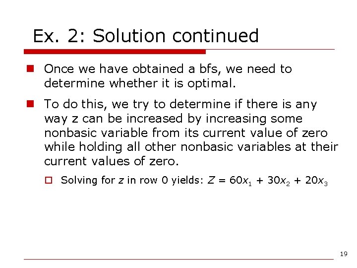
Ex. 2: Solution continued n Once we have obtained a bfs, we need to determine whether it is optimal. n To do this, we try to determine if there is any way z can be increased by increasing some nonbasic variable from its current value of zero while holding all other nonbasic variables at their current values of zero. o Solving for z in row 0 yields: Z = 60 x 1 + 30 x 2 + 20 x 3 19

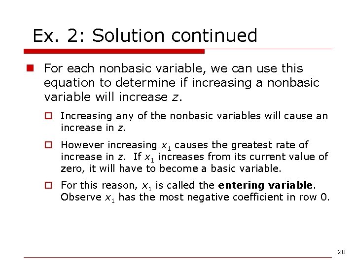
Ex. 2: Solution continued n For each nonbasic variable, we can use this equation to determine if increasing a nonbasic variable will increase z. o Increasing any of the nonbasic variables will cause an increase in z. o However increasing x 1 causes the greatest rate of increase in z. If x 1 increases from its current value of zero, it will have to become a basic variable. o For this reason, x 1 is called the entering variable. Observe x 1 has the most negative coefficient in row 0. 20

Ex. 2: Solution continued n Next choose the entering variable to be the nonbasic variable with the most negative coefficient in row 0. n Goal is to make x 1 as large as possible but as it increases, the current basic variables will change value. Thus, increasing x 1 may cause a basic variable to become negative. n This means to keep all the basic variables nonnegative, the largest we can make x 1 is min {6, 5, 4} = 4. 21

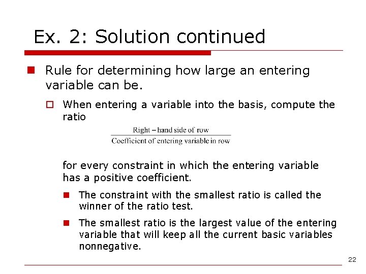
Ex. 2: Solution continued n Rule for determining how large an entering variable can be. o When entering a variable into the basis, compute the ratio for every constraint in which the entering variable has a positive coefficient. n The constraint with the smallest ratio is called the winner of the ratio test. n The smallest ratio is the largest value of the entering variable that will keep all the current basic variables nonnegative. 22

Ex. 2: Solution continued n Always make the entering variable a basic variable in a row that wins the ratio test. n To make x 1 a basic variable in row 3, we use elementary row operations (EROs) to make x 1 have a coefficient of 1 in row 3 and a coefficient of 0 in all other rows. o This procedure is called pivoting on row 3; and row 3 is called the pivot row. o The final result is that x 1 replaces s 3 as the basic variable for row 3. The term in the pivot row that involves the entering basic variable is called the pivot term. 23

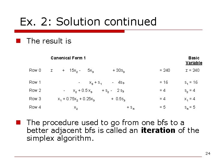
Ex. 2: Solution continued n The result is Canonical Form 1 Row 0 z + 15 x 2 - Row 1 Row 2 - Basic Variable 5 x 3 + 30 s 3 = 240 z = 240 - 4 s 3 = 16 s 1 = 16 + s 2 - 2 s 3 =4 s 2 = 4 + 0. 5 s 3 =4 x 1 = 4 =5 s 4 = 5 x 3 + s 1 x 2 + 0. 5 x 3 Row 3 x 1 + 0. 75 x 2 + 0. 25 x 3 Row 4 x 2 + s 4 n The procedure used to go from one bfs to a better adjacent bfs is called an iteration of the simplex algorithm. 24

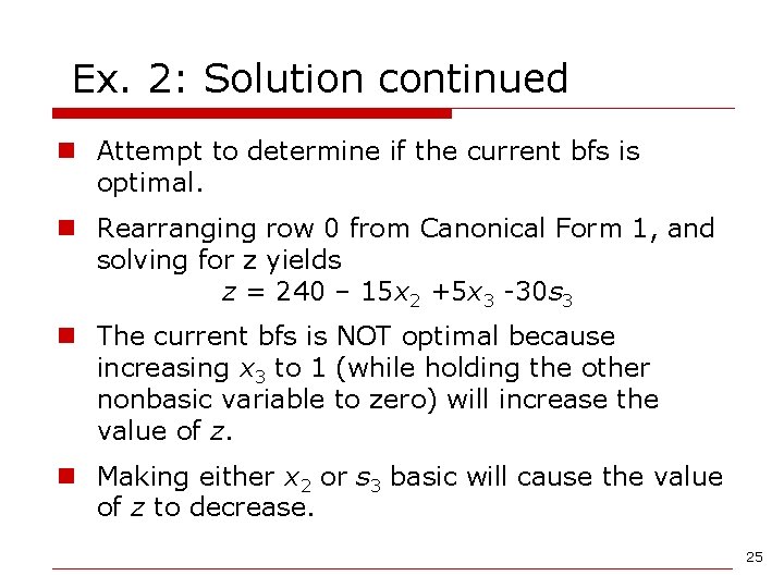
Ex. 2: Solution continued n Attempt to determine if the current bfs is optimal. n Rearranging row 0 from Canonical Form 1, and solving for z yields z = 240 – 15 x 2 +5 x 3 -30 s 3 n The current bfs is NOT optimal because increasing x 3 to 1 (while holding the other nonbasic variable to zero) will increase the value of z. n Making either x 2 or s 3 basic will cause the value of z to decrease. 25

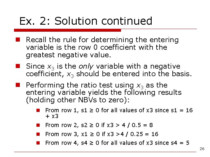
Ex. 2: Solution continued n Recall the rule for determining the entering variable is the row 0 coefficient with the greatest negative value. n Since x 3 is the only variable with a negative coefficient, x 3 should be entered into the basis. n Performing the ratio test using x 3 as the entering variable yields the following results (holding other NBVs to zero): n From row 1, s 1 ≥ 0 for all values of x 3 since s 1 = 16 + x 3 n From row 2, s 2 ≥ 0 if x 3 > 4 / 0. 5 = 8 n From row 3, x 1 ≥ 0 if x 3 >4 / 0. 25 = 16 n From row 4, s 4 ≥ 0 for all values of x 3 since s 4 = 5 26

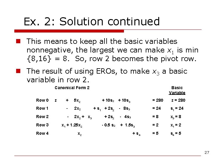
Ex. 2: Solution continued n This means to keep all the basic variables nonnegative, the largest we can make x 1 is min {8, 16} = 8. So, row 2 becomes the pivot row. n The result of using EROs, to make x 3 a basic variable in row 2. Canonical Form 2 Row 0 z + 5 x 2 Row 1 - 2 x 2 Row 2 - 2 x 2 + x 3 Row 3 x 1 + 1. 25 x 2 Row 4 x 2 Basic Variable + 10 s 2 + 10 s 3 = 280 z = 280 + s 1 + 2 s 2 - 8 s 3 = 24 s 1 = 24 + 2 s 2 - 4 s 3 =8 x 3 = 8 + 1. 5 s 3 =2 x 1 = 2 =5 s 4 = 5 - 0. 5 s 2 + s 4 27

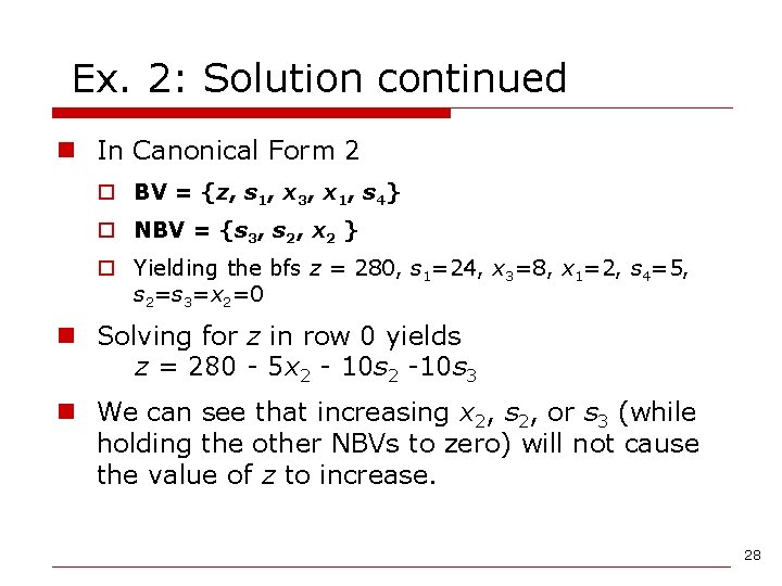
Ex. 2: Solution continued n In Canonical Form 2 o BV = {z, s 1, x 3, x 1, s 4} o NBV = {s 3, s 2, x 2 } o Yielding the bfs z = 280, s 1=24, x 3=8, x 1=2, s 4=5, s 2=s 3=x 2=0 n Solving for z in row 0 yields z = 280 - 5 x 2 - 10 s 2 -10 s 3 n We can see that increasing x 2, s 2, or s 3 (while holding the other NBVs to zero) will not cause the value of z to increase. 28

Ex. 2: Solution continued n The solution at the end of iteration 2 is therefore optimal. The following rule can be applied to determine whether a canonical form’s bfs is optimal. o A canonical form is optimal (for a max problem) if each nonbasic variable has a nonnegative coefficient in the canonical form’s row 0. 29

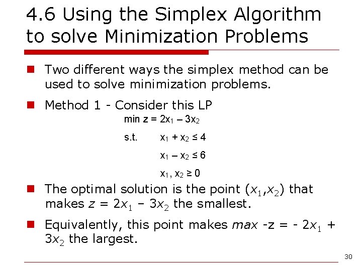
4. 6 Using the Simplex Algorithm to solve Minimization Problems n Two different ways the simplex method can be used to solve minimization problems. n Method 1 - Consider this LP min z = 2 x 1 – 3 x 2 s. t. x 1 + x 2 ≤ 4 x 1 – x 2 ≤ 6 x 1, x 2 ≥ 0 n The optimal solution is the point (x 1, x 2) that makes z = 2 x 1 – 3 x 2 the smallest. n Equivalently, this point makes max -z = - 2 x 1 + 3 x 2 the largest. 30

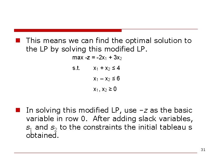
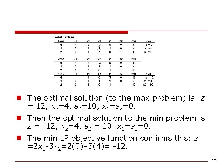
n This means we can find the optimal solution to the LP by solving this modified LP. max -z = -2 x 1 + 3 x 2 s. t. x 1 + x 2 ≤ 4 x 1 – x 2 ≤ 6 x 1, x 2 ≥ 0 n In solving this modified LP, use –z as the basic variable in row 0. After adding slack variables, s 1 and s 2 to the constraints the initial tableau s obtained. 31

n The optimal solution (to the max problem) is -z = 12, x 2=4, s 2=10, x 1=s 2=0. n Then the optimal solution to the min problem is z = -12, x 2=4, s 2 = 10, x 1=s 2=0. n The min LP objective function confirms this: z =2 x 1 -3 x 2=2(0)– 3(4)= -12. 32

n In summary, multiply the objective function for the min problem by -1 and solve the problem as a maximization problem with the objective function –z. n The optimal solution to the max problem will give you the optimal solution for to the min problem. n Remember that (optimal z-value for the min problem) = - (optimal z-value for the max problem). 33

n Method 2 - A simple modification of the simplex algorithm can be used to solve min problems directly. o Modify step 3 of the simplex algorithm n If all nonbasic variables (NBV) in row 0 have nonpositive coefficients, the current bfs is optimal. n If any nonbasic variable has a positive coefficient, choose the variable with the “most positive” coefficient in row 0 as the entering variable. n This modification of the simplex algorithm works because increasing a nonbasic variable (NBV) with a positive coefficient in row 0 will decrease z. 34