Markov Chains 1 Markov Chains A Markov Chain

Markov Chains 1

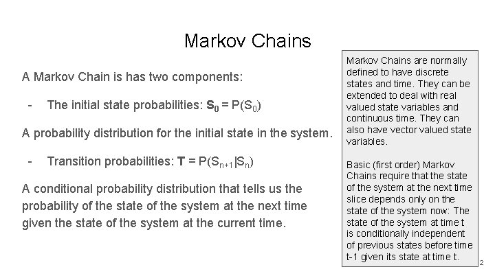
Markov Chains A Markov Chain is has two components: - The initial state probabilities: S 0 = P(S 0) A probability distribution for the initial state in the system. - Transition probabilities: T = P(Sn+1|Sn) A conditional probability distribution that tells us the probability of the state of the system at the next time given the state of the system at the current time. Markov Chains are normally defined to have discrete states and time. They can be extended to deal with real valued state variables and continuous time. They can also have vector valued state variables. Basic (first order) Markov Chains require that the state of the system at the next time slice depends only on the state of the system now: The state of the system at time t is conditionally independent of previous states before time t-1 given its state at time t. 2

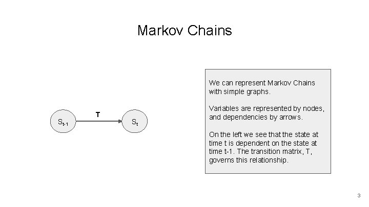
Markov Chains We can represent Markov Chains with simple graphs. St-1 T St Variables are represented by nodes, and dependencies by arrows. On the left we see that the state at time t is dependent on the state at time t-1. The transition matrix, T, governs this relationship. 3

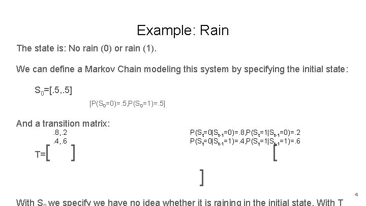
Example: Rain The state is: No rain (0) or rain (1). We can define a Markov Chain modeling this system by specifying the initial state: S 0=[. 5, . 5] [P(S 0=0)=. 5, P(S 0=1)=. 5] And a transition matrix: T= [ . 8, . 2. 4, . 6 ] P(St=0|St-1=0)=. 8, P(St=1|St-1=0)=. 2 P(St=0|St-1=1)=. 4, P(St=1|St-1=1)=. 6 [ ] 4

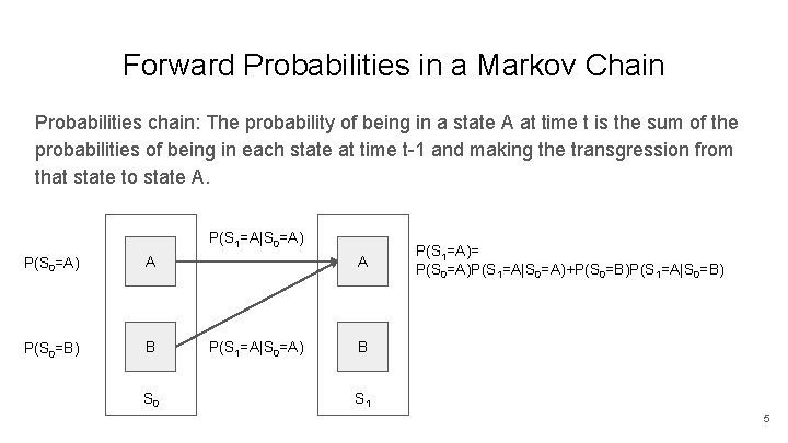
Forward Probabilities in a Markov Chain Probabilities chain: The probability of being in a state A at time t is the sum of the probabilities of being in each state at time t-1 and making the transgression from that state to state A. P(S 1=A|S 0=A) P(S 0=A) A P(S 0=B) B S 0 A P(S 1=A|S 0=A) P(S 1=A)= P(S 0=A)P(S 1=A|S 0=A)+P(S 0=B)P(S 1=A|S 0=B) B S 1 5

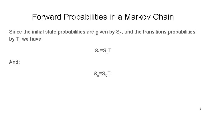
Forward Probabilities in a Markov Chain Since the initial state probabilities are given by S 0, and the transitions probabilities by T, we have: S 1=S 0 T And: Sn=S 0 Tn 6

Full Example For a full example of the predicting future state distributions in a Markov Chain (by iteratively calculating probability values, not just a one line matrix equation), see the Markov Examples pdf. 7

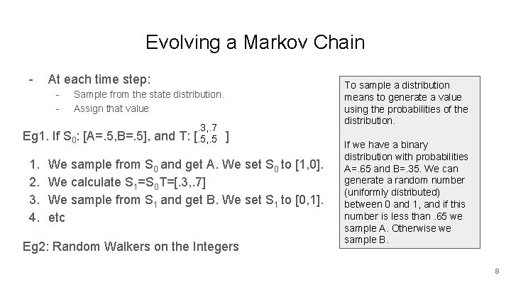
Evolving a Markov Chain - At each time step: - Sample from the state distribution. Assign that value. 3, . 7 Eg 1. If S 0: [A=. 5, B=. 5], and T: [. 5, . 5 ] 1. 2. 3. 4. We sample from S 0 and get A. We set S 0 to [1, 0]. We calculate S 1=S 0 T=[. 3, . 7] We sample from S 1 and get B. We set S 1 to [0, 1]. etc Eg 2: Random Walkers on the Integers To sample a distribution means to generate a value using the probabilities of the distribution. If we have a binary distribution with probabilities A=. 65 and B=. 35. We can generate a random number (uniformly distributed) between 0 and 1, and if this number is less than. 65 we sample A. Otherwise we sample B. 8

Long Run Distribution A Markov Chain gives a distribution for the next state given the current state. Associated with a Markov Chain is another distribution: The long-run (or steadystate) distribution. This is the proportion of time the system will spend in different states is it is evolved forever. If we can set up a Markov Chain that has a specific (but unknown) long-run distribution, we can estimate this distribution by evolving the Markov Chain. We will return to this idea in a later lecture. 9

Hidden Markov Models 10

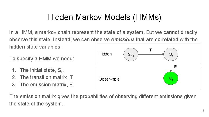
Hidden Markov Models (HMMs) In a HMM, a markov chain represent the state of a system. But we cannot directly observe this state. Instead, we can observe emissions that are correlated with the hidden state variables. To specify a HMM we need: 1. The initial state, S 0. 2. The transition matrix, T. 3. The emission matrix, E. Hidden St-1 T St E Observable Ot The emission matrix gives the probabilities of observing different emissions given the state of the system. 11

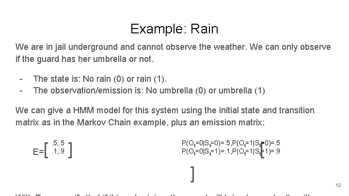
Example: Rain We are in jail underground and cannot observe the weather. We can only observe if the guard has her umbrella or not. - The state is: No rain (0) or rain (1). The observation/emission is: No umbrella (0) or umbrella (1) We can give a HMM model for this system using the initial state and transition matrix as in the Markov Chain example, plus an emission matrix: E= [ . 5, . 5. 1, . 9 ] [ P(Ot=0|St=0)=. 5, P(Ot=1|St=0)=. 5 P(Ot=0|St=1)=. 1, P(Ot=1|St=1)=. 9 ] 12

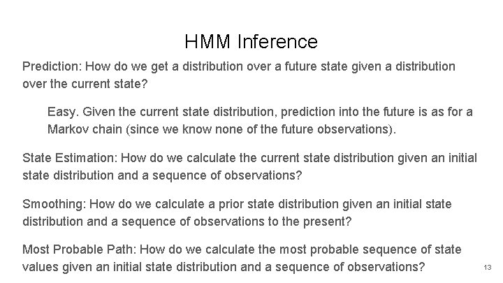
HMM Inference Prediction: How do we get a distribution over a future state given a distribution over the current state? Easy. Given the current state distribution, prediction into the future is as for a Markov chain (since we know none of the future observations). State Estimation: How do we calculate the current state distribution given an initial state distribution and a sequence of observations? Smoothing: How do we calculate a prior state distribution given an initial state distribution and a sequence of observations to the present? Most Probable Path: How do we calculate the most probable sequence of state values given an initial state distribution and a sequence of observations? 13

State Estimation Used to predict current state of system given initial state and observations up until present. 14

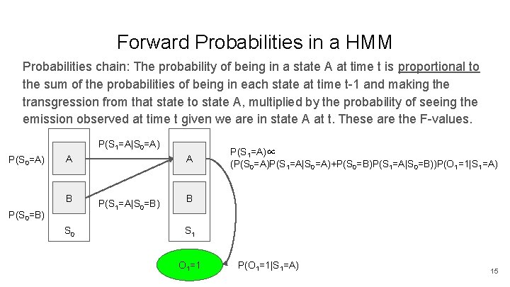
Forward Probabilities in a HMM Probabilities chain: The probability of being in a state A at time t is proportional to the sum of the probabilities of being in each state at time t-1 and making the transgression from that state to state A, multiplied by the probability of seeing the emission observed at time t given we are in state A at t. These are the F-values. P(S 1=A|S 0=A) P(S 0=A) A B P(S 0=B) S 0 A P(S 1=A|S 0=B) P(S 1=A)∝ (P(S 0=A)P(S 1=A|S 0=A)+P(S 0=B)P(S 1=A|S 0=B))P(O 1=1|S 1=A) B S 1 O 1=1 P(O 1=1|S 1=A) 15

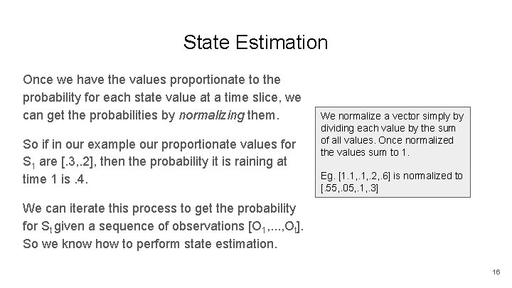
State Estimation Once we have the values proportionate to the probability for each state value at a time slice, we can get the probabilities by normalizing them. So if in our example our proportionate values for S 1 are [. 3, . 2], then the probability it is raining at time 1 is. 4. We normalize a vector simply by dividing each value by the sum of all values. Once normalized the values sum to 1. Eg. [1. 1, . 2, . 6] is normalized to [. 55, . 05, . 1, . 3] We can iterate this process to get the probability for St given a sequence of observations [O 1, . . . , Ot]. So we know how to perform state estimation. 16

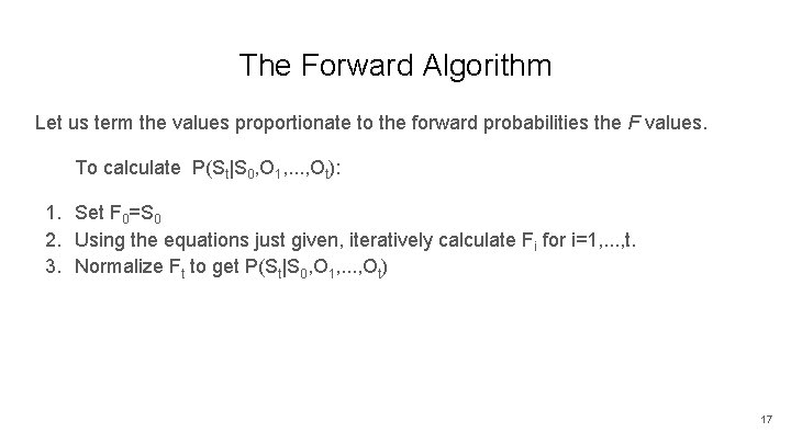
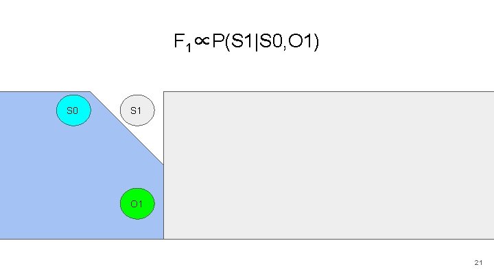
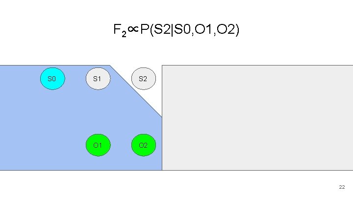
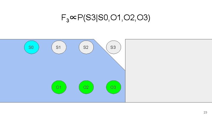
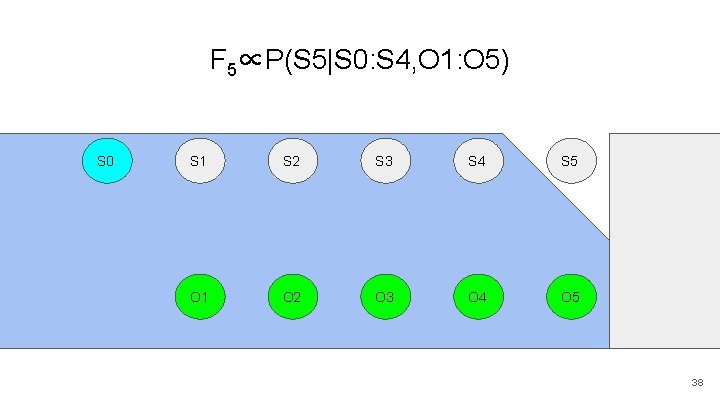
The Forward Algorithm Let us term the values proportionate to the forward probabilities the F values. To calculate P(St|S 0, O 1, . . . , Ot): 1. Set F 0=S 0 2. Using the equations just given, iteratively calculate Fi for i=1, . . . , t. 3. Normalize Ft to get P(St|S 0, O 1, . . . , Ot) 17

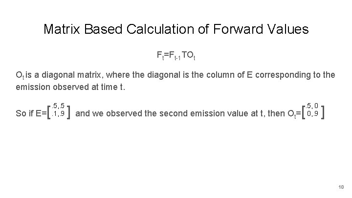
Matrix Based Calculation of Forward Values Ft=Ft-1 TOt Ot is a diagonal matrix, where the diagonal is the column of E corresponding to the emission observed at time t. So if E= [ . 5, . 5. 1, . 9 ] and we observed the second emission value at t, then O =[ t . 5, 0 0, . 9 ] 18

System from time 0 to time 5 S 0 S 1 S 2 S 3 S 4 S 5 O 1 O 2 O 3 O 4 O 5 19

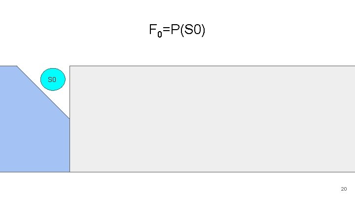
F 0=P(S 0) S 0 S 1 S 2 S 3 S 4 S 5 O 1 O 2 O 3 O 4 O 5 20

F 1∝P(S 1|S 0, O 1) S 0 S 1 S 2 S 3 S 4 S 5 O 1 O 2 O 3 O 4 O 5 21

F 2∝P(S 2|S 0, O 1, O 2) S 0 S 1 S 2 S 3 S 4 S 5 O 1 O 2 O 3 O 4 O 5 22

F 3∝P(S 3|S 0, O 1, O 2, O 3) S 0 S 1 S 2 S 3 S 4 S 5 O 1 O 2 O 3 O 4 O 5 23

F 4∝P(S 4|S 0, O 1, O 2, O 3, O 4) S 0 S 1 S 2 S 3 S 4 S 5 O 1 O 2 O 3 O 4 O 5 24

F 5∝P(S 5|S 0: S 4, O 1: O 5) S 0 S 1 S 2 S 3 S 4 S 5 O 1 O 2 O 3 O 4 O 5 25

Full Example For a full example of the forward algorithm, with values and iterative calculations of the F values, see the Markov Examples pdf. 26

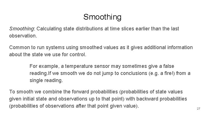
Smoothing: Calculating state distributions at time slices earlier than the last observation. Common to run systems using smoothed values as it gives additional information about the state we use for control. For example, a temperature sensor may sometimes give a false reading. If we smooth we do not jump to conclusions (e. g. a fire!) from a single reading. To smooth we combine the forward probabilities (probabilities of state values given initial state and observations up to that point) with backward probabilities (probabilities of observations after that point given value). 27

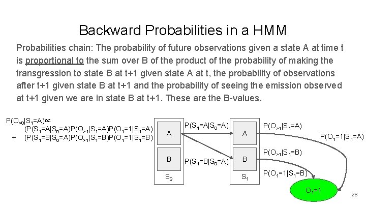
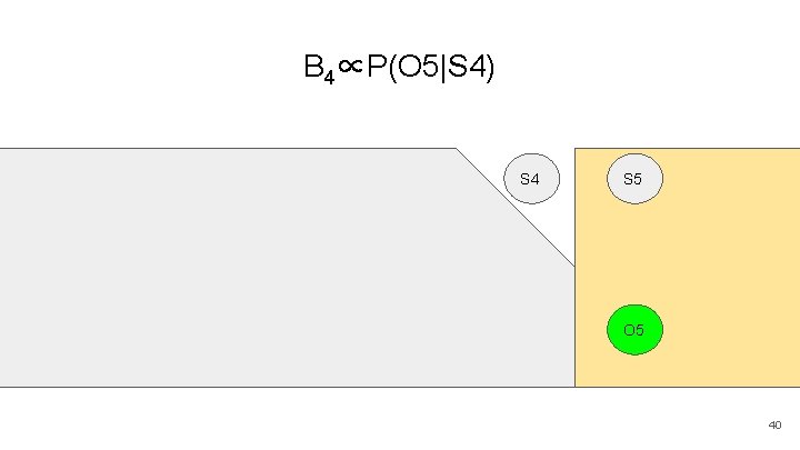
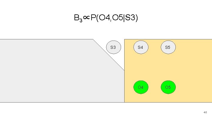
Backward Probabilities in a HMM Probabilities chain: The probability of future observations given a state A at time t is proportional to the sum over B of the product of the probability of making the transgression to state B at t+1 given state A at t, the probability of observations after t+1 given state B at t+1 and the probability of seeing the emission observed at t+1 given we are in state B at t+1. These are the B-values. P(O>0|S 1=A)∝ (P(S 1=A|S 0=A)P(O>1|S 1=A)P(O 1=1|S 1=A) + (P(S 1=B|S 0=A)P(O>1|S 1=B)P(O 1=1|S 1=B) A B S 0 P(S 1=A|S 0=A) P(S 1=B|S 0=A) A B S 1 P(O>1|S 1=A) P(O 1=1|S 1=A) P(O>1|S 1=B) P(O 1=1|S 1=B) O 1=1 28

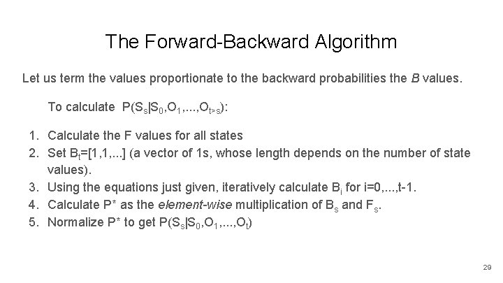
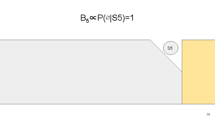
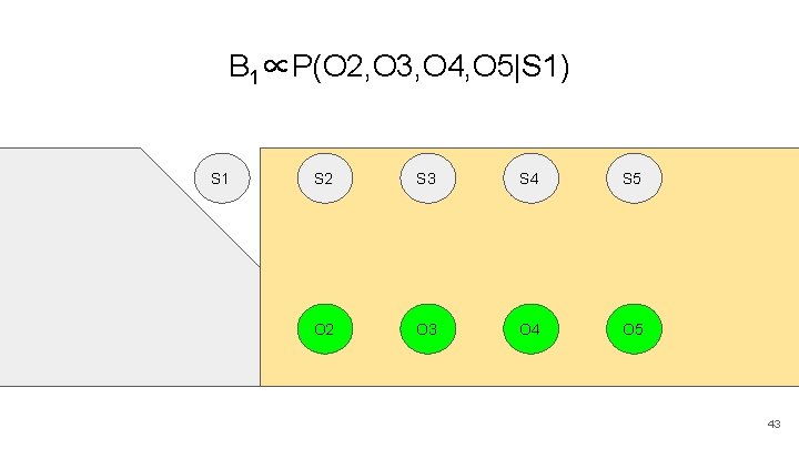
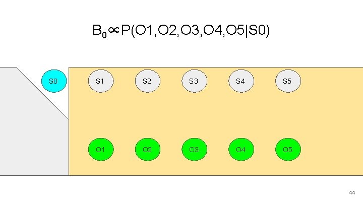
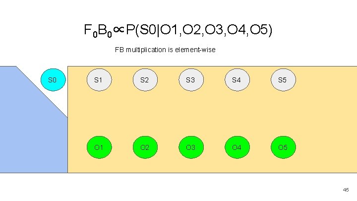
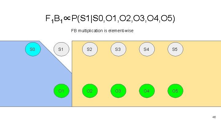
The Forward-Backward Algorithm Let us term the values proportionate to the backward probabilities the B values. To calculate P(Ss|S 0, O 1, . . . , Ot>s): 1. Calculate the F values for all states 2. Set Bt=[1, 1, . . . ] (a vector of 1 s, whose length depends on the number of state values). 3. Using the equations just given, iteratively calculate Bi for i=0, . . . , t-1. 4. Calculate P* as the element-wise multiplication of Bs and Fs. 5. Normalize P* to get P(Ss|S 0, O 1, . . . , Ot) 29

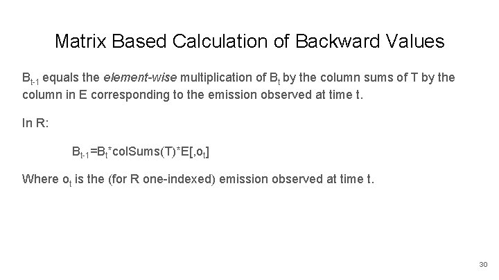
Matrix Based Calculation of Backward Values Bt-1 equals the element-wise multiplication of Bt by the column sums of T by the column in E corresponding to the emission observed at time t. In R: Bt-1=Bt*col. Sums(T)*E[, ot] Where ot is the (for R one-indexed) emission observed at time t. 30

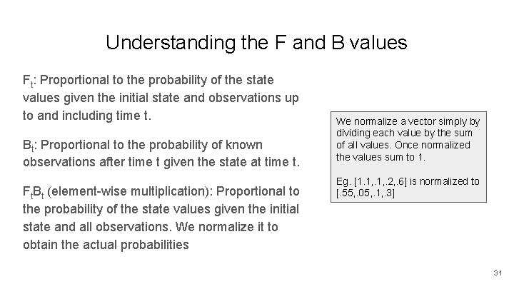
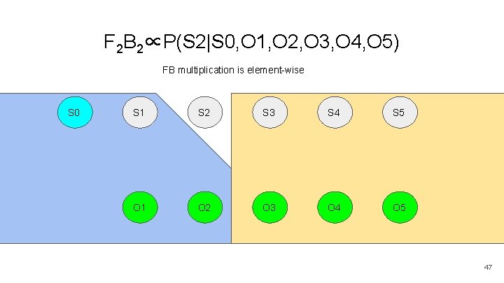
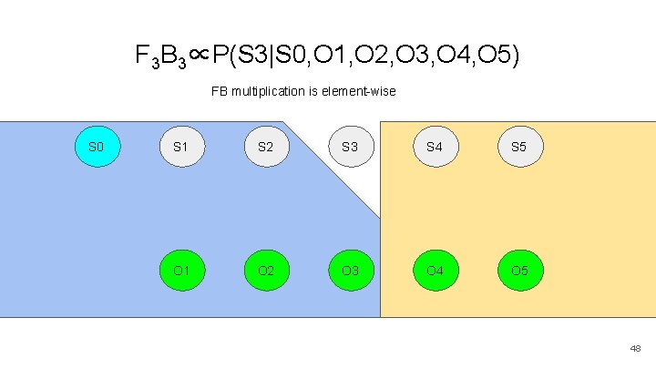
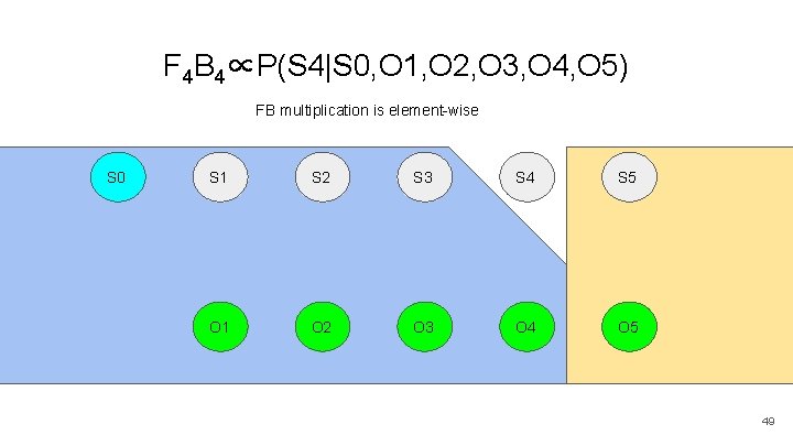
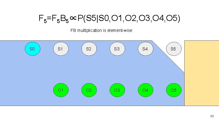
Understanding the F and B values Ft: Proportional to the probability of the state values given the initial state and observations up to and including time t. Bt: Proportional to the probability of known observations after time t given the state at time t. Ft. Bt (element-wise multiplication): Proportional to the probability of the state values given the initial state and all observations. We normalize it to obtain the actual probabilities We normalize a vector simply by dividing each value by the sum of all values. Once normalized the values sum to 1. Eg. [1. 1, . 2, . 6] is normalized to [. 55, . 05, . 1, . 3] 31

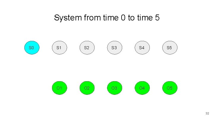
System from time 0 to time 5 S 0 S 1 S 2 S 3 S 4 S 5 O 1 O 2 O 3 O 4 O 5 32

F 0∝P(S 0) S 0 S 1 S 2 S 3 S 4 S 5 O 1 O 2 O 3 O 4 O 5 33

F 1∝P(S 1|S 0, O 1) S 0 S 1 S 2 S 3 S 4 S 5 O 1 O 2 O 3 O 4 O 5 34

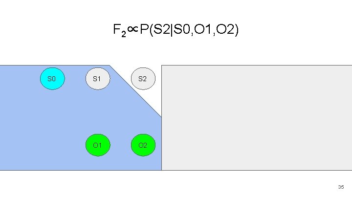
F 2∝P(S 2|S 0, O 1, O 2) S 0 S 1 S 2 S 3 S 4 S 5 O 1 O 2 O 3 O 4 O 5 35

F 3∝P(S 3|S 0, O 1, O 2, O 3) S 0 S 1 S 2 S 3 S 4 S 5 O 1 O 2 O 3 O 4 O 5 36

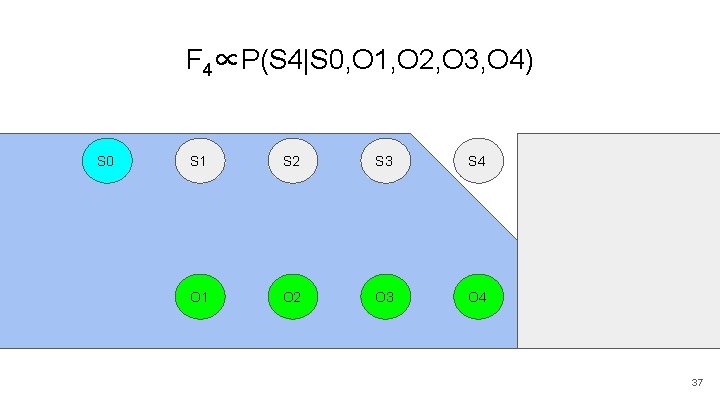
F 4∝P(S 4|S 0, O 1, O 2, O 3, O 4) S 0 S 1 S 2 S 3 S 4 S 5 O 1 O 2 O 3 O 4 O 5 37

F 5∝P(S 5|S 0: S 4, O 1: O 5) S 0 S 1 S 2 S 3 S 4 S 5 O 1 O 2 O 3 O 4 O 5 38

B 5∝P(∅|S 5)=1 S 0 S 1 S 2 S 3 S 4 S 5 O 1 O 2 O 3 O 4 O 5 39

B 4∝P(O 5|S 4) S 0 S 1 S 2 S 3 S 4 S 5 O 1 O 2 O 3 O 4 O 5 40

B 3∝P(O 4, O 5|S 3) S 0 S 1 S 2 S 3 S 4 S 5 O 1 O 2 O 3 O 4 O 5 41

B 2∝P(O 3, O 4, O 5|S 2) S 0 S 1 S 2 S 3 S 4 S 5 O 1 O 2 O 3 O 4 O 5 42

B 1∝P(O 2, O 3, O 4, O 5|S 1) S 0 S 1 S 2 S 3 S 4 S 5 O 1 O 2 O 3 O 4 O 5 43

B 0∝P(O 1, O 2, O 3, O 4, O 5|S 0) S 0 S 1 S 2 S 3 S 4 S 5 O 1 O 2 O 3 O 4 O 5 44

F 0 B 0∝P(S 0|O 1, O 2, O 3, O 4, O 5) FB multiplication is element-wise S 0 S 1 S 2 S 3 S 4 S 5 O 1 O 2 O 3 O 4 O 5 45

F 1 B 1∝P(S 1|S 0, O 1, O 2, O 3, O 4, O 5) FB multiplication is element-wise S 0 S 1 S 2 S 3 S 4 S 5 O 1 O 2 O 3 O 4 O 5 46

F 2 B 2∝P(S 2|S 0, O 1, O 2, O 3, O 4, O 5) FB multiplication is element-wise S 0 S 1 S 2 S 3 S 4 S 5 O 1 O 2 O 3 O 4 O 5 47

F 3 B 3∝P(S 3|S 0, O 1, O 2, O 3, O 4, O 5) FB multiplication is element-wise S 0 S 1 S 2 S 3 S 4 S 5 O 1 O 2 O 3 O 4 O 5 48

F 4 B 4∝P(S 4|S 0, O 1, O 2, O 3, O 4, O 5) FB multiplication is element-wise S 0 S 1 S 2 S 3 S 4 S 5 O 1 O 2 O 3 O 4 O 5 49

F 5=F 5 B 5∝P(S 5|S 0, O 1, O 2, O 3, O 4, O 5) FB multiplication is element-wise S 0 S 1 S 2 S 3 S 4 S 5 O 1 O 2 O 3 O 4 O 5 50

Full Example For a full example of the forward-backward algorithm, with values and iterative calculations of the F and B values, see the Markov Examples pdf. 51

Most Probable Path: The Viterbi Algorithm Calculate the most probable sequence of state values given an initial distribution and a sequence of observations. - Use in a surprisingly large number of real-world problems. Basis theorem: If the most probable path from A to C passes through B, then it is the concatenation of the most probable path from A to B with the most probable path from B to C. NB This algorithm is related very closely to the dynamic programming for path finding algorithm in the online lecture: Lecture 2: Search Basics. If you have not read this lecture, you should do so as soon as possible. 52

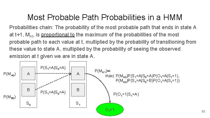
Most Probable Path Probabilities in a HMM Probabilities chain: The probability of the most probable path that ends in state A at t+1, MAt, is proportional to the maximum of the probabilities of the most probable path to each value at t, multiplied by the probability of transitioning from these value to state A, multiplied by the probability of seeing the observed emission at t given we are in state A. P(S 1=A|S 0=A) P(MA 0) A B P(MB 0) S 0 A P(S 1=A|S 0=A) B P(MA 1)∝ max( P(MA 0)P(S 1=A|S 0=A)P(O 1=A|S 1=1), P(MA 0)P(S 1=A|S 0=B)P(O 1=A|S 1=1)) P(O 1=1|S 1=A) S 1 O 1=1 53

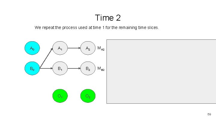
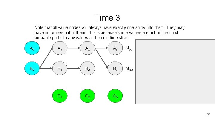
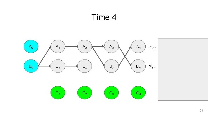
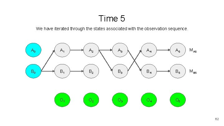
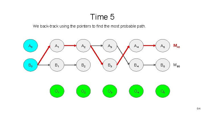
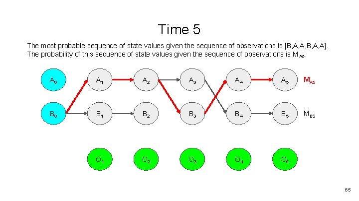
The Viterbi Algorithm 1. Set Mx 0=P(S 0=x) from the initial state distribution specification 2. Iteratively progress through the time slice: a. Calculate the M value for each state value. b. Add a pointer from that state value to the state value of the preceding time slice that gave the maximal value. 3. On the final time slice, chose the state value with the largest M value. Follow the pointers backwards through the time slices to find the most probable path given the initial state distribution and the sequence of observations. The probability of the most probable path is the M values of its terminal node. 54

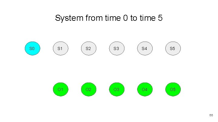
System from time 0 to time 5 S 0 S 1 S 2 S 3 S 4 S 5 O 1 O 2 O 3 O 4 O 5 55

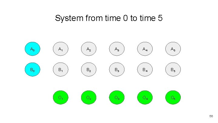
System from time 0 to time 5 A 0 A 1 A 2 A 3 A 4 A 5 B 0 B 1 B 2 B 3 B 4 B 5 O 1 O 2 O 3 O 4 O 5 56

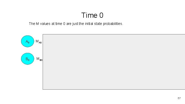
Time 0 The M values at time 0 are just the initial state probabilities. A 0 MA 0 A 1 A 2 A 3 A 4 A 5 B 0 MB 0 B 1 B 2 B 3 B 4 B 5 O 1 O 2 O 3 O 4 O 5 57

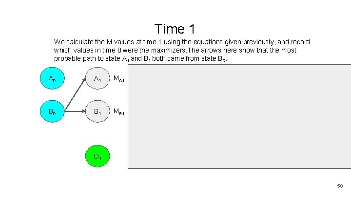
Time 1 We calculate the M values at time 1 using the equations given previously, and record which values in time 0 were the maximizers. The arrows here show that the most probable path to state A 1 and B 1 both came from state B 0. A 0 A 1 MA 1 A 2 A 3 A 4 A 5 B 0 B 1 MB 1 B 2 B 3 B 4 B 5 O 2 O 3 O 4 O 5 O 1 58

Time 2 We repeat the process used at time 1 for the remaining time slices. A 0 A 1 A 2 MA 2 A 3 A 4 A 5 B 0 B 1 B 2 MB 2 B 3 B 4 B 5 O 1 O 2 O 3 O 4 O 5 59

Time 3 Note that all value nodes will always have exactly one arrow into them. They may have no arrows out of them. This is because some values are not on the most probable paths to any values at the next time slice. A 0 A 1 A 2 A 3 MA 3 A 4 A 5 B 0 B 1 B 2 B 3 MB 3 B 4 B 5 O 1 O 2 O 3 O 4 O 5 60

Time 4 A 0 A 1 A 2 A 3 A 4 MA 4 A 5 B 0 B 1 B 2 B 3 B 4 MB 4 B 5 O 1 O 2 O 3 O 4 O 5 61

Time 5 We have iterated through the states associated with the observation sequence. A 0 A 1 A 2 A 3 A 4 A 5 MA 5 B 0 B 1 B 2 B 3 B 4 B 5 MB 5 O 1 O 2 O 3 O 4 O 5 62

Time 5 Let us assume MA 5 > MB 5. A 0 A 1 A 2 A 3 A 4 A 5 MA 5 B 0 B 1 B 2 B 3 B 4 B 5 MB 5 O 1 O 2 O 3 O 4 O 5 63

Time 5 We back-track using the pointers to find the most probable path. A 0 A 1 A 2 A 3 A 4 A 5 MA 5 B 0 B 1 B 2 B 3 B 4 B 5 MB 5 O 1 O 2 O 3 O 4 O 5 64

Time 5 The most probable sequence of state values given the sequence of observations is [B, A, A, B, A, A]. The probability of this sequence of state values given the sequence of observations is MA 5. A 0 A 1 A 2 A 3 A 4 A 5 MA 5 B 0 B 1 B 2 B 3 B 4 B 5 MB 5 O 1 O 2 O 3 O 4 O 5 65

Full Example For a full example of the Viterbi algorithm, with values and iterative calculations of the M values, see the Markov Examples pdf. Note that in this example the M values are not labelled M values. So p 01 in the example is M 01 in the M notation. 66