Dynamic programming A method of solving a large

Dynamic programming A method of solving a large problem by dividing it up into smaller subproblems and solving those, then putting them together to solve the larger problem. Can often have more than one way of aligning two sequences, dynamic programming allows backtracking and testing of various options. The path that most effectively links together the subproblems into an optimal solution is selected as the final alignment. Needs to be based on statistics of scoring system and probability thresholds set May still end up with a few solutions of equal scores – Ultimately need a biologically relevant answer.

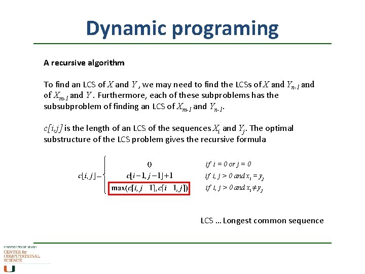
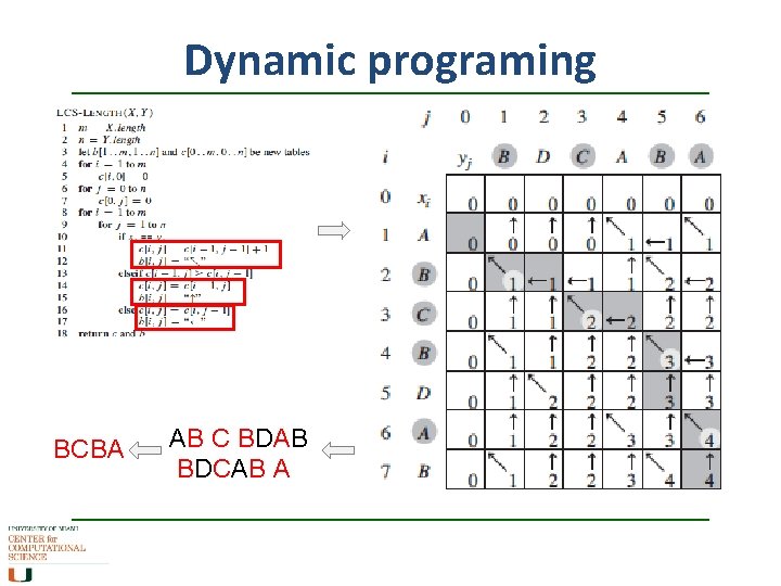
Dynamic programing A recursive algorithm To find an LCS of X and Y , we may need to find the LCSs of X and Yn-1 and of Xm-1 and Y. Furthermore, each of these subproblems has the subsubproblem of finding an LCS of Xm-1 and Yn-1. c[i, j] is the length of an LCS of the sequences Xi and Yj. The optimal substructure of the LCS problem gives the recursive formula if i = 0 or j = 0 if i, j > 0 and xi = yj if i, j > 0 and xi ≠ yj LCS … Longest common sequence

Dynamic programing BCBA AB C BDAB BDCAB A

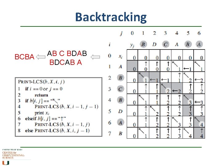
Backtracking BCBA AB C BDAB BDCAB A

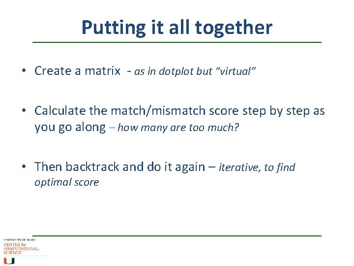
Putting it all together • Create a matrix - as in dotplot but “virtual” • Calculate the match/mismatch score step by step as you go along – how many are too much? • Then backtrack and do it again – iterative, to find optimal score

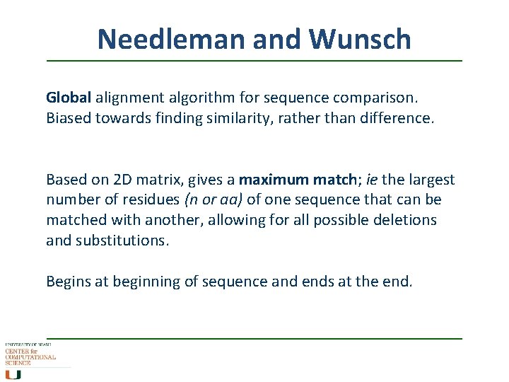
Needleman and Wunsch Global alignment algorithm for sequence comparison. Biased towards finding similarity, rather than difference. Based on 2 D matrix, gives a maximum match; ie the largest number of residues (n or aa) of one sequence that can be matched with another, allowing for all possible deletions and substitutions. Begins at beginning of sequence and ends at the end.

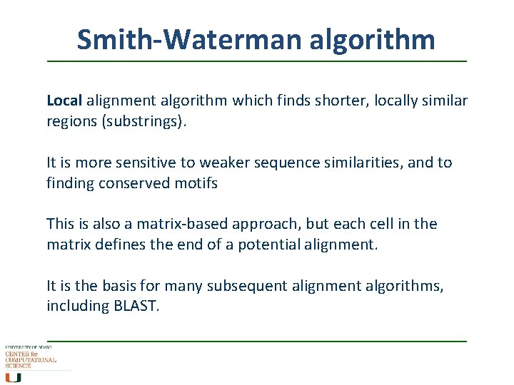
Smith-Waterman algorithm Local alignment algorithm which finds shorter, locally similar regions (substrings). It is more sensitive to weaker sequence similarities, and to finding conserved motifs This is also a matrix-based approach, but each cell in the matrix defines the end of a potential alignment. It is the basis for many subsequent alignment algorithms, including BLAST.

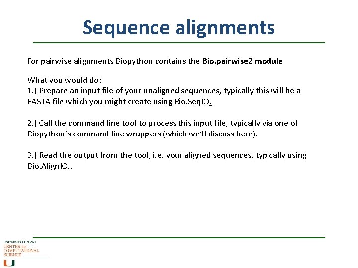
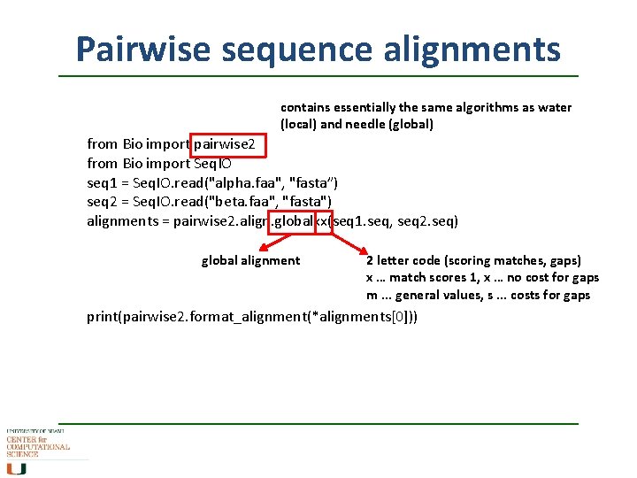
Sequence alignments For pairwise alignments Biopython contains the Bio. pairwise 2 module What you would do: 1. ) Prepare an input file of your unaligned sequences, typically this will be a FASTA file which you might create using Bio. Seq. IO. 2. ) Call the command line tool to process this input file, typically via one of Biopython’s command line wrappers (which we’ll discuss here). 3. ) Read the output from the tool, i. e. your aligned sequences, typically using Bio. Align. IO. .

Pairwise sequence alignments contains essentially the same algorithms as water (local) and needle (global) from Bio import pairwise 2 from Bio import Seq. IO seq 1 = Seq. IO. read("alpha. faa", "fasta”) seq 2 = Seq. IO. read("beta. faa", "fasta") alignments = pairwise 2. align. globalxx(seq 1. seq, seq 2. seq) global alignment 2 letter code (scoring matches, gaps) x … match scores 1, x … no cost for gaps m. . . general values, s. . . costs for gaps print(pairwise 2. format_alignment(*alignments[0]))

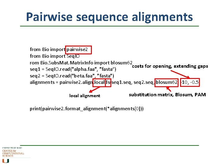
Pairwise sequence alignments from Bio import pairwise 2 from Bio import Seq. IO rom Bio. Subs. Matrix. Info import blosum 62 costs for opening, extending gaps seq 1 = Seq. IO. read("alpha. faa", "fasta”) seq 2 = Seq. IO. read("beta. faa", "fasta") alignments = pairwise 2. align. localds(seq 1. seq, seq 2. seq, blosum 62, -10, -0. 5) local alignment substitution matrix, Blosum, PAM print(pairwise 2. format_alignment(*alignments[0]))

Problem with N-W and S-W They are exhaustive, with stringent statistical thresholds As the databases got larger, these began to take too long – computational constraints Need a program that runs an algorithm that is based on dynamic programming (substrings) but uses a heuristic approach (takes assumptions, quicker, not as refined). Therefore can deal with comparing a sequence against 100 million others in a relatively short time… the bigger the database, the more optimal the results.

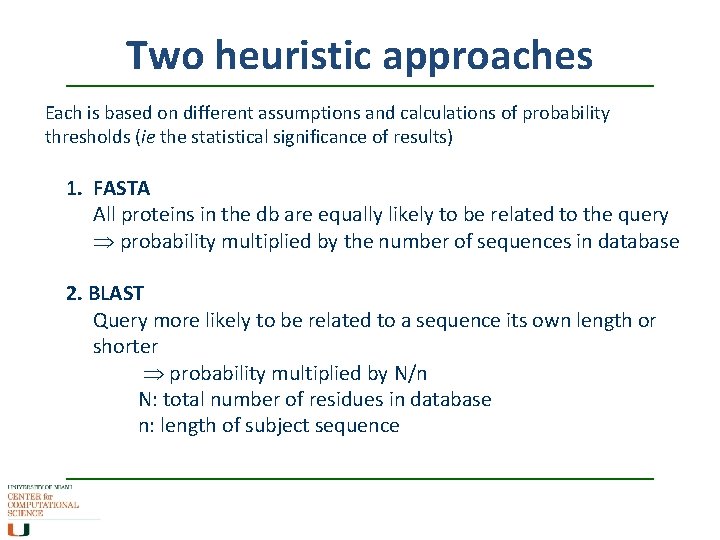
Two heuristic approaches Each is based on different assumptions and calculations of probability thresholds (ie the statistical significance of results) 1. FASTA All proteins in the db are equally likely to be related to the query probability multiplied by the number of sequences in database 2. BLAST Query more likely to be related to a sequence its own length or shorter probability multiplied by N/n N: total number of residues in database n: length of subject sequence

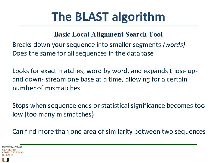
The BLAST algorithm Basic Local Alignment Search Tool Breaks down your sequence into smaller segments (words) Does the same for all sequences in the database Looks for exact matches, word by word, and expands those upand down- stream one base at a time, allowing for a certain number of mismatches Stops when sequence ends or statistical significance becomes too low (too many mismatches) Can find more than one area of similarity between two sequences

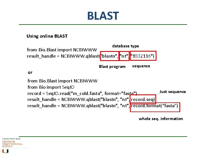
BLAST Using online BLAST database type from Bio. Blast import NCBIWWW result_handle = NCBIWWW. qblast("blastn", "nt", "8332116") Blast program sequence or from Bio. Blast import NCBIWWW from Bio import Seq. IO Just sequence record = Seq. IO. read("m_cold. fasta", format="fasta") result_handle = NCBIWWW. qblast("blastn", "nt", record. seq) result_handle = NCBIWWW. qblast("blastn", "nt", record. format(“fasta”) whole seq. information

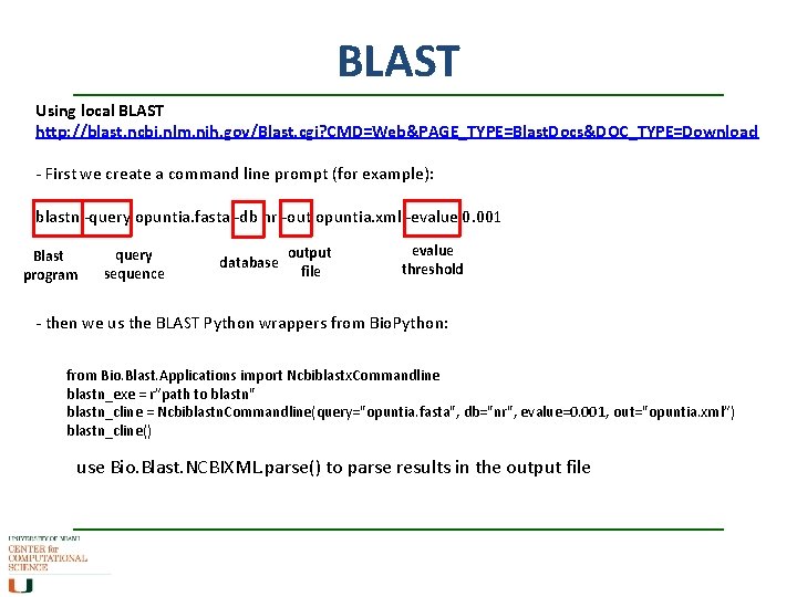
BLAST Using local BLAST http: //blast. ncbi. nlm. nih. gov/Blast. cgi? CMD=Web&PAGE_TYPE=Blast. Docs&DOC_TYPE=Download - First we create a command line prompt (for example): blastn -query opuntia. fasta -db nr -out opuntia. xml -evalue 0. 001 Blast program query sequence database output file evalue threshold - then we us the BLAST Python wrappers from Bio. Python: from Bio. Blast. Applications import Ncbiblastx. Commandline blastn_exe = r”path to blastn" blastn_cline = Ncbiblastn. Commandline(query="opuntia. fasta", db="nr", evalue=0. 001, out="opuntia. xml”) blastn_cline() use Bio. Blast. NCBIXML. parse() to parse results in the output file

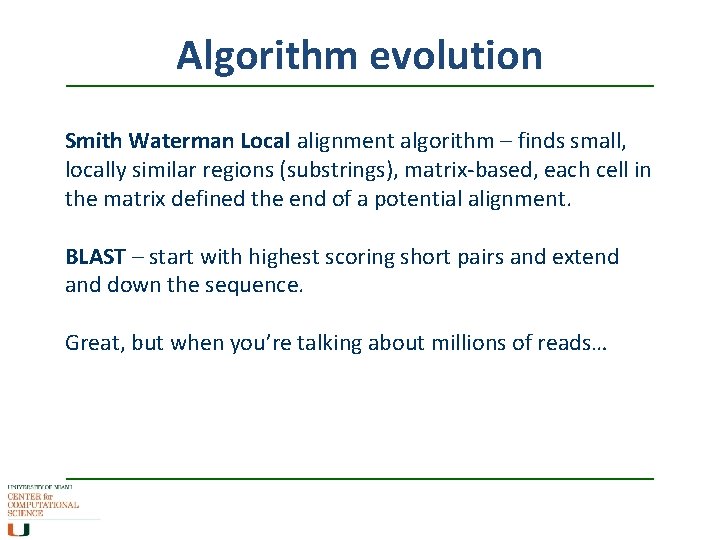
Algorithm evolution Smith Waterman Local alignment algorithm – finds small, locally similar regions (substrings), matrix-based, each cell in the matrix defined the end of a potential alignment. BLAST – start with highest scoring short pairs and extend and down the sequence. Great, but when you’re talking about millions of reads…