MODULE4 DYNAMIC PROGRAMMING Dynamic Programming Dynamic Programming is

![Floyd’s Algorithm (pseudocode and analysis) Time efficiency: Θ(n 3) If D[i, k] + D[k, Floyd’s Algorithm (pseudocode and analysis) Time efficiency: Θ(n 3) If D[i, k] + D[k,](https://slidetodoc.com/presentation_image_h2/8c64bd176572e15b90d7fc2a71c9293c/image-12.jpg)
![Knapsack Problem by DP (pseudocode) Algorithm DPKnapsack(w[1. . n], v[1. . n], W) var Knapsack Problem by DP (pseudocode) Algorithm DPKnapsack(w[1. . n], v[1. . n], W) var](https://slidetodoc.com/presentation_image_h2/8c64bd176572e15b90d7fc2a71c9293c/image-22.jpg)
![0 -1 Knapsack Memory Function Algorithm MFKnapsack(i, W) if V[i, W] < 0 if 0 -1 Knapsack Memory Function Algorithm MFKnapsack(i, W) if V[i, W] < 0 if](https://slidetodoc.com/presentation_image_h2/8c64bd176572e15b90d7fc2a71c9293c/image-42.jpg)


- Slides: 44

MODULE-4 DYNAMIC PROGRAMMING

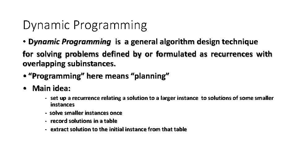
Dynamic Programming • Dynamic Programming is a general algorithm design technique for solving problems defined by or formulated as recurrences with overlapping subinstances. • “Programming” here means “planning” • Main idea: - set up a recurrence relating a solution to a larger instance to solutions of some smaller instances - solve smaller instances once - record solutions in a table - extract solution to the initial instance from that table

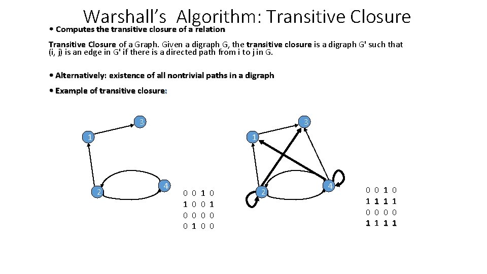
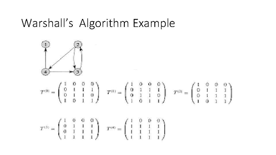
Warshall’s Algorithm: Transitive Closure • Computes the transitive closure of a relation Transitive Closure of a Graph. Given a digraph G, the transitive closure is a digraph G' such that (i, j) is an edge in G' if there is a directed path from i to j in G. • Alternatively: existence of all nontrivial paths in a digraph • Example of transitive closure: 3 3 1 1 2 4 0 1 0 0 0 1 1 0 0 2 4 0 1 0 1 1 1 0 1 0 1

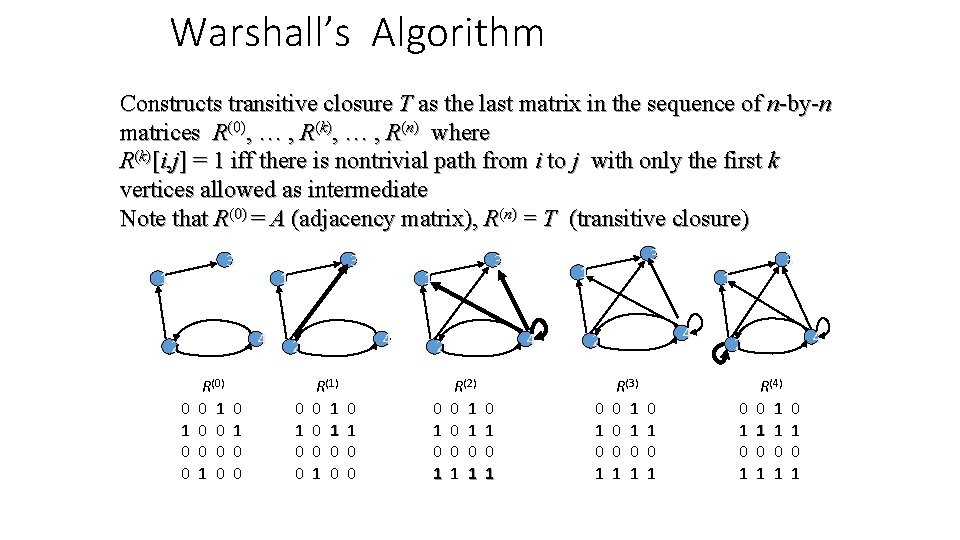
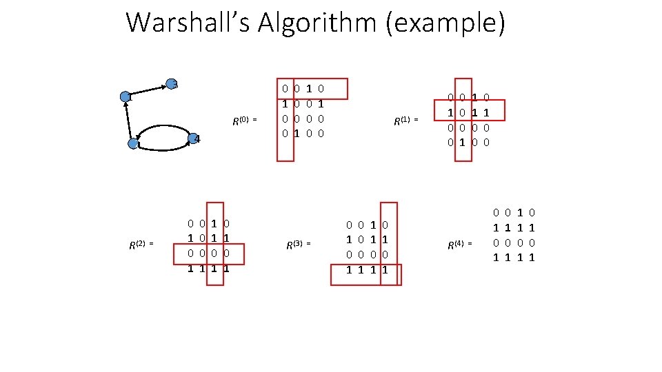
Warshall’s Algorithm Constructs transitive closure T as the last matrix in the sequence of n-by-n matrices R(0), … , R(k), … , R(n) where R(k)[i, j] = 1 iff there is nontrivial path from i to j with only the first k vertices allowed as intermediate Note that R(0) = A (adjacency matrix), R(n) = T (transitive closure) 3 1 1 4 2 0 1 0 0 R(0) 0 1 0 0 3 0 1 0 0 1 4 2 R(1) 0 1 0 0 3 0 1 1 4 2 R(2) 0 1 0 0 1 1 0 1 3 3 1 4 2 0 1 R(3) 0 1 0 0 1 1 0 1 4 2 0 1 R(4) 0 1 1 1 0 0 1 1 0 1

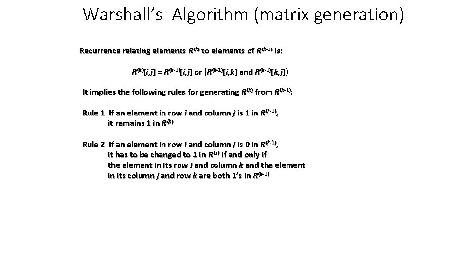
Warshall’s Algorithm (matrix generation) Recurrence relating elements R(k) to elements of R(k-1) is: R(k)[i, j] = R(k-1)[i, j] or (R(k-1)[i, k] and R(k-1)[k, j]) It implies the following rules for generating R(k) from R(k-1): Rule 1 If an element in row i and column j is 1 in R(k-1), it remains 1 in R(k) Rule 2 If an element in row i and column j is 0 in R(k-1), it has to be changed to 1 in R(k) if and only if the element in its row i and column k and the element in its column j and row k are both 1’s in R(k-1)

Warshall’s Algorithm Example

Warshall’s Algorithm (example) 3 1 R(0) = 4 2 R(2) = 0 1 0 0 0 1 1 1 0 1 0 1 0 0 0 1 1 0 0 0 R(3) = 0 1 0 0 R(1) = 0 1 0 0 0 1 1 1 0 1 0 1 0 0 0 1 R(4) = 1 1 0 0 0 1 0 1 0 1 1 1 0 1 0 1

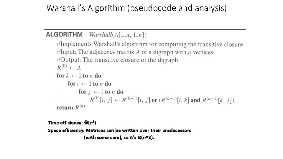
Warshall’s Algorithm (pseudocode and analysis) Time efficiency: Θ(n 3) Space efficiency: Matrices can be written over their predecessors (with some care), so it’s Θ(n^2).

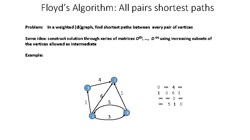
Floyd’s Algorithm: All pairs shortest paths Problem: In a weighted (di)graph, find shortest paths between every pair of vertices Same idea: construct solution through series of matrices D(0), …, D (n) using increasing subsets of the vertices allowed as intermediate Example: 4 3 1 6 1 2 0 ∞ 4 ∞ 1 0 6 3 ∞ ∞ 0 ∞ ∞ 5 1 0 1 5 3 4

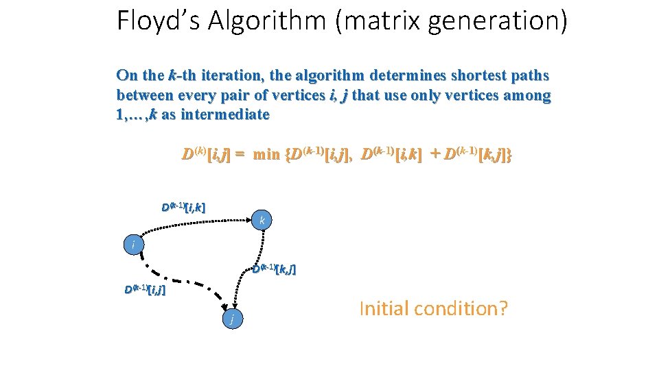
Floyd’s Algorithm (matrix generation) On the k-th iteration, the algorithm determines shortest paths between every pair of vertices i, j that use only vertices among 1, …, k as intermediate D(k)[i, j] = min {D(k-1)[i, j], D(k-1)[i, k] + D(k-1)[k, j]} D(k-1)[i, k] k i D(k-1)[k, j] D(k-1)[i, j] j Initial condition?

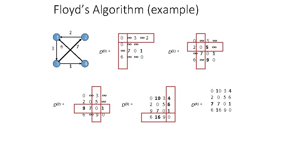
Floyd’s Algorithm (example) 2 1 6 3 3 D(2) = 2 7 1 D(0) = 0 0 ∞ 6 ∞ ∞ 7 ∞ 3 ∞ 2 ∞ 0 1 ∞ 0 D(1) = 4 0 2 9 6 ∞ 0 7 ∞ 3 5 0 9 ∞ ∞ 1 0 D(3) = 0 2 9 6 10 0 7 16 3 5 0 9 4 6 1 0 0 2 ∞ 6 ∞ 0 7 ∞ D(4) = 3 5 0 9 ∞ ∞ 1 0 0 2 7 6 10 0 7 16 3 5 0 9 4 6 1 0
![Floyds Algorithm pseudocode and analysis Time efficiency Θn 3 If Di k Dk Floyd’s Algorithm (pseudocode and analysis) Time efficiency: Θ(n 3) If D[i, k] + D[k,](https://slidetodoc.com/presentation_image_h2/8c64bd176572e15b90d7fc2a71c9293c/image-12.jpg)
Floyd’s Algorithm (pseudocode and analysis) Time efficiency: Θ(n 3) If D[i, k] + D[k, j] < D[i, j] then P[i, j] k Space efficiency: Matrices can be written over their predecessors Note: Works on graphs with negative edges but without negative cycles. Shortest paths themselves can be found, too. How?

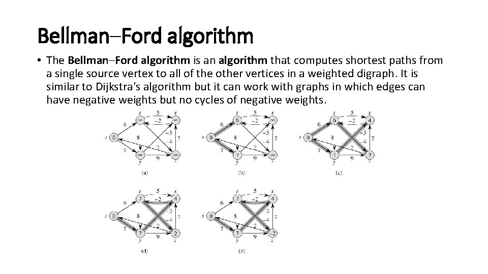
Bellman–Ford algorithm • The Bellman–Ford algorithm is an algorithm that computes shortest paths from a single source vertex to all of the other vertices in a weighted digraph. It is similar to Dijkstra's algorithm but it can work with graphs in which edges can have negative weights but no cycles of negative weights.

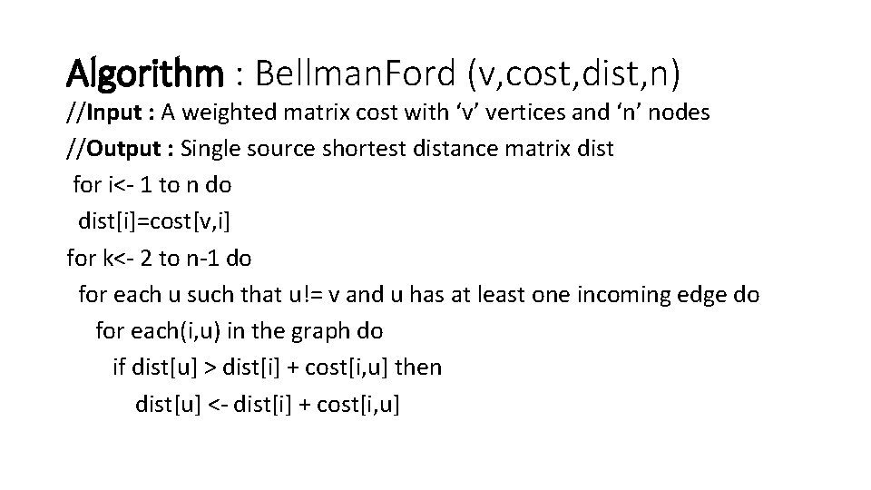
Algorithm : Bellman. Ford (v, cost, dist, n) //Input : A weighted matrix cost with ‘v’ vertices and ‘n’ nodes //Output : Single source shortest distance matrix dist for i<- 1 to n do dist[i]=cost[v, i] for k<- 2 to n-1 do for each u such that u!= v and u has at least one incoming edge do for each(i, u) in the graph do if dist[u] > dist[i] + cost[i, u] then dist[u] <- dist[i] + cost[i, u]

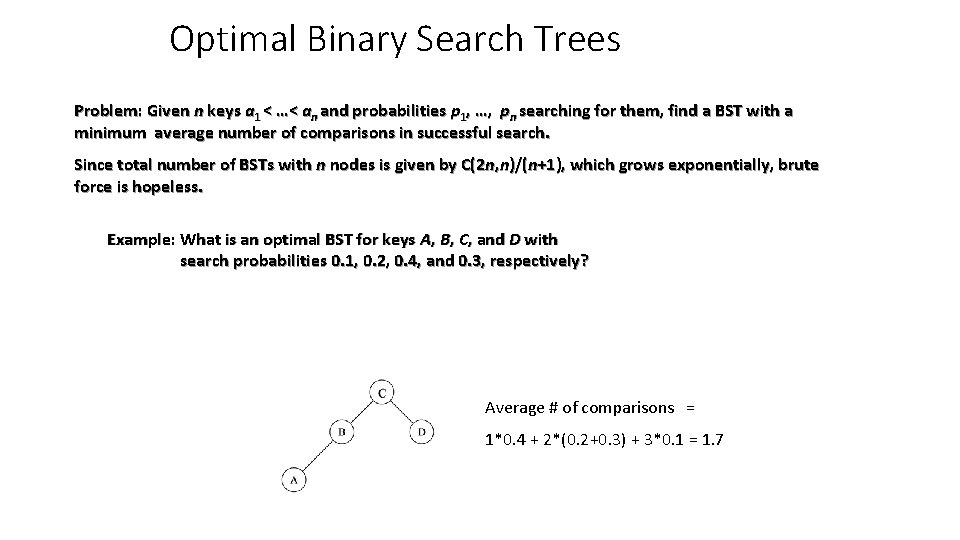
Optimal Binary Search Trees Problem: Given n keys a 1 < …< an and probabilities p 1, …, pn searching for them, find a BST with a minimum average number of comparisons in successful search. Since total number of BSTs with n nodes is given by C(2 n, n)/(n+1), which grows exponentially, brute force is hopeless. Example: What is an optimal BST for keys A, B, C, and D with search probabilities 0. 1, 0. 2, 0. 4, and 0. 3, respectively? Average # of comparisons = 1*0. 4 + 2*(0. 2+0. 3) + 3*0. 1 = 1. 7

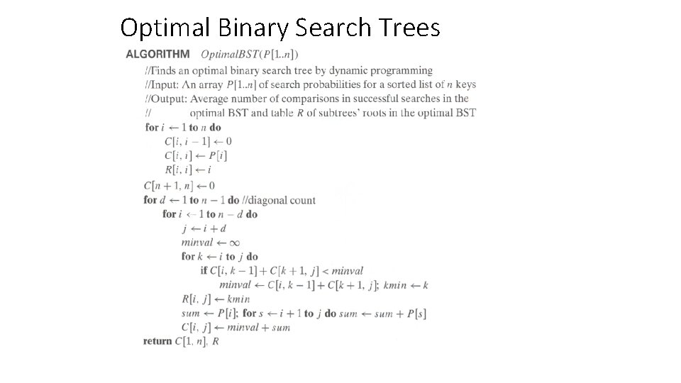
Optimal Binary Search Trees

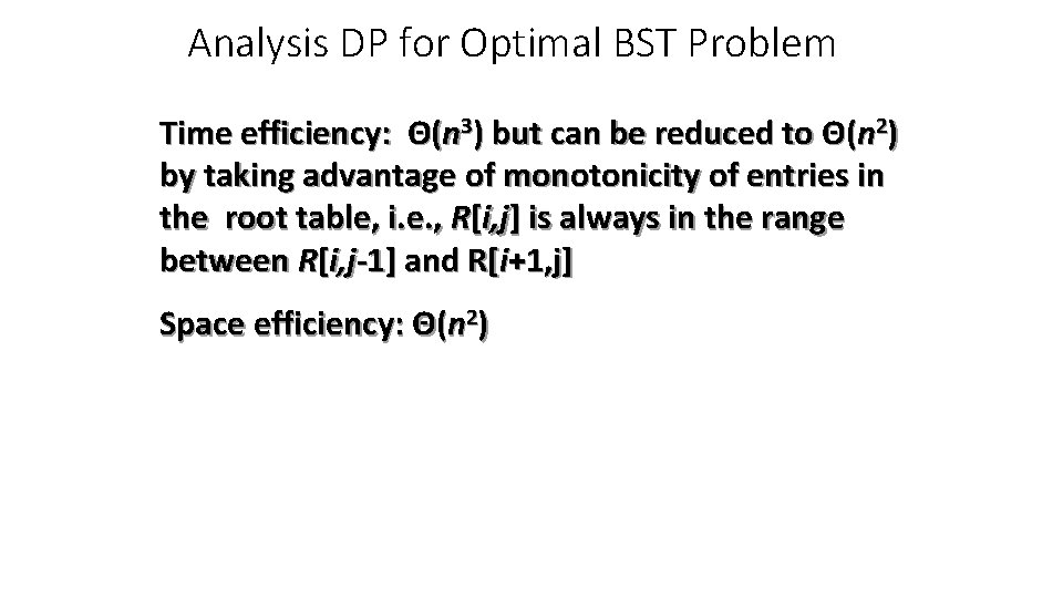
Analysis DP for Optimal BST Problem Time efficiency: Θ(n 3) but can be reduced to Θ(n 2) by taking advantage of monotonicity of entries in the root table, i. e. , R[i, j] is always in the range between R[i, j-1] and R[i+1, j] Space efficiency: Θ(n 2)

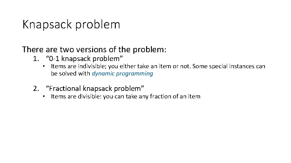
Knapsack problem There are two versions of the problem: 1. “ 0 -1 knapsack problem” • Items are indivisible; you either take an item or not. Some special instances can be solved with dynamic programming 2. “Fractional knapsack problem” • Items are divisible: you can take any fraction of an item

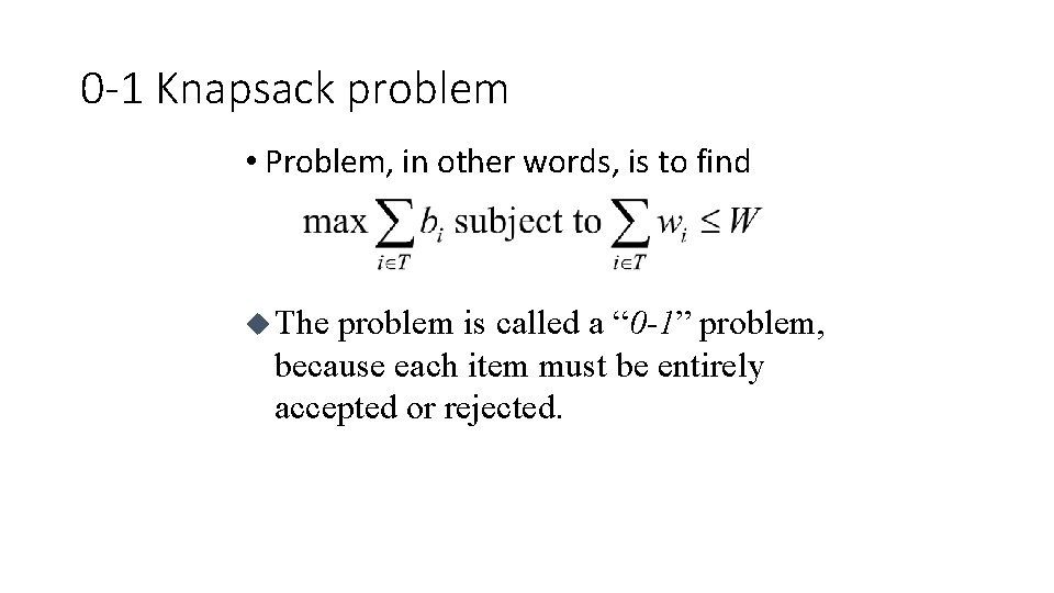
0 -1 Knapsack problem • Problem, in other words, is to find u The problem is called a “ 0 -1” problem, because each item must be entirely accepted or rejected.

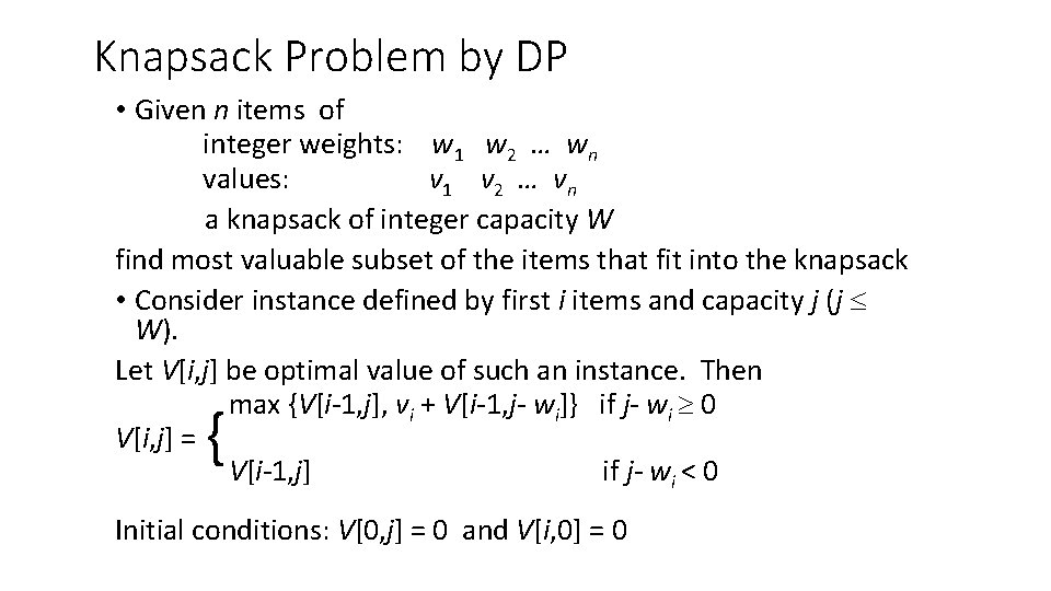
Knapsack Problem by DP • Given n items of integer weights: w 1 w 2 … wn values: v 1 v 2 … v n a knapsack of integer capacity W find most valuable subset of the items that fit into the knapsack • Consider instance defined by first i items and capacity j (j W). Let V[i, j] be optimal value of such an instance. Then max {V[i-1, j], vi + V[i-1, j- wi]} if j- wi 0 V[i, j] = V[i-1, j] if j- wi < 0 { Initial conditions: V[0, j] = 0 and V[i, 0] = 0

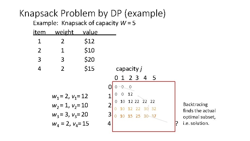
Knapsack Problem by DP (example) Example: Knapsack of capacity W = 5 item weight value 1 2 $12 2 1 $10 3 3 $20 4 2 $15 capacity j 0 1 2 3 4 5 0 0 w 1 = 2, v 1= 12 1 0 0 12 0 10 12 22 22 22 w 2 = 1, v 2= 10 2 0 10 12 22 30 32 w 3 = 3, v 3= 20 3 0 10 15 25 30 37 w 4 = 2, v 4= 15 4 ? Backtracing finds the actual optimal subset, i. e. solution.
![Knapsack Problem by DP pseudocode Algorithm DPKnapsackw1 n v1 n W var Knapsack Problem by DP (pseudocode) Algorithm DPKnapsack(w[1. . n], v[1. . n], W) var](https://slidetodoc.com/presentation_image_h2/8c64bd176572e15b90d7fc2a71c9293c/image-22.jpg)
Knapsack Problem by DP (pseudocode) Algorithm DPKnapsack(w[1. . n], v[1. . n], W) var V[0. . n, 0. . W], P[1. . n, 1. . W]: int for j : = 0 to W do V[0, j] : = 0 Running time and space: for i : = 0 to n do O(n. W). V[i, 0] : = 0 for i : = 1 to n do for j : = 1 to W do if w[i] j and v[i] + V[i-1, j-w[i]] > V[i-1, j] then V[i, j] : = v[i] + V[i-1, j-w[i]]; P[i, j] : = j-w[i] else V[i, j] : = V[i-1, j]; P[i, j] : = j return V[n, W] and the optimal subset by backtracing

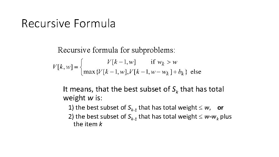
Recursive Formula Recursive formula for subproblems: It means, that the best subset of Sk that has total weight w is: 1) the best subset of Sk-1 that has total weight w, or 2) the best subset of Sk-1 that has total weight w-wk plus the item k

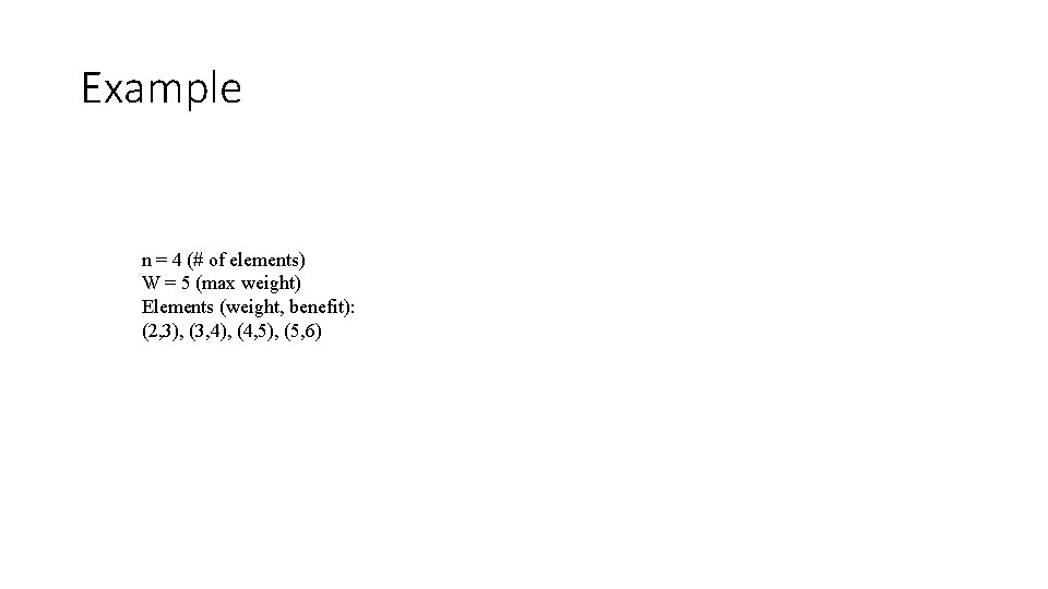
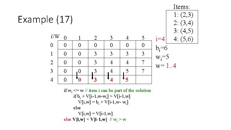
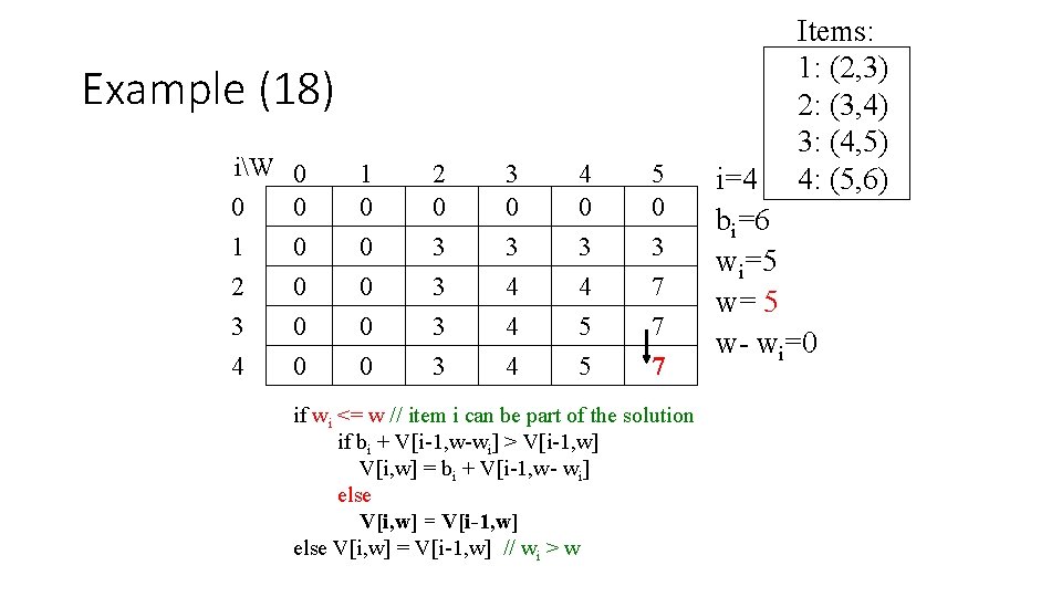
Example n = 4 (# of elements) W = 5 (max weight) Elements (weight, benefit): (2, 3), (3, 4), (4, 5), (5, 6)

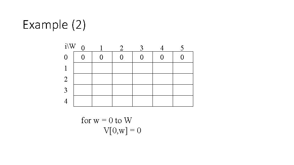
Example (2) iW 0 0 0 1 2 3 4 1 0 2 0 3 0 for w = 0 to W V[0, w] = 0 4 0 5 0

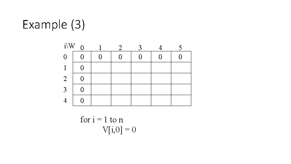
Example (3) iW 0 1 2 3 4 0 0 0 1 0 2 0 for i = 1 to n V[i, 0] = 0 3 0 4 0 5 0

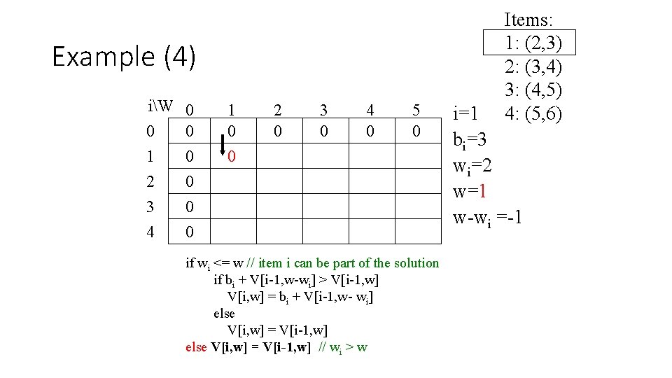
Example (4) iW 0 1 2 3 4 0 0 0 1 0 0 2 0 3 0 4 0 5 0 if wi <= w // item i can be part of the solution if bi + V[i-1, w-wi] > V[i-1, w] V[i, w] = bi + V[i-1, w- wi] else V[i, w] = V[i-1, w] // wi > w Items: 1: (2, 3) 2: (3, 4) 3: (4, 5) 4: (5, 6) i=1 bi=3 wi=2 w=1 w-wi =-1

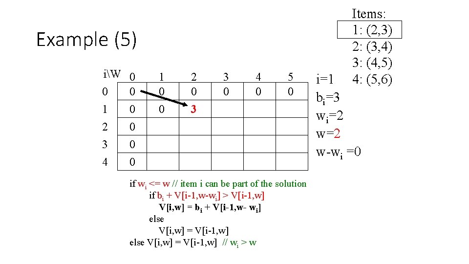
Example (5) iW 0 0 0 1 0 2 0 3 0 4 0 1 0 0 2 0 3 3 0 4 0 5 0 if wi <= w // item i can be part of the solution if bi + V[i-1, w-wi] > V[i-1, w] V[i, w] = bi + V[i-1, w- wi] else V[i, w] = V[i-1, w] // wi > w Items: 1: (2, 3) 2: (3, 4) 3: (4, 5) 4: (5, 6) i=1 bi=3 wi=2 w-wi =0

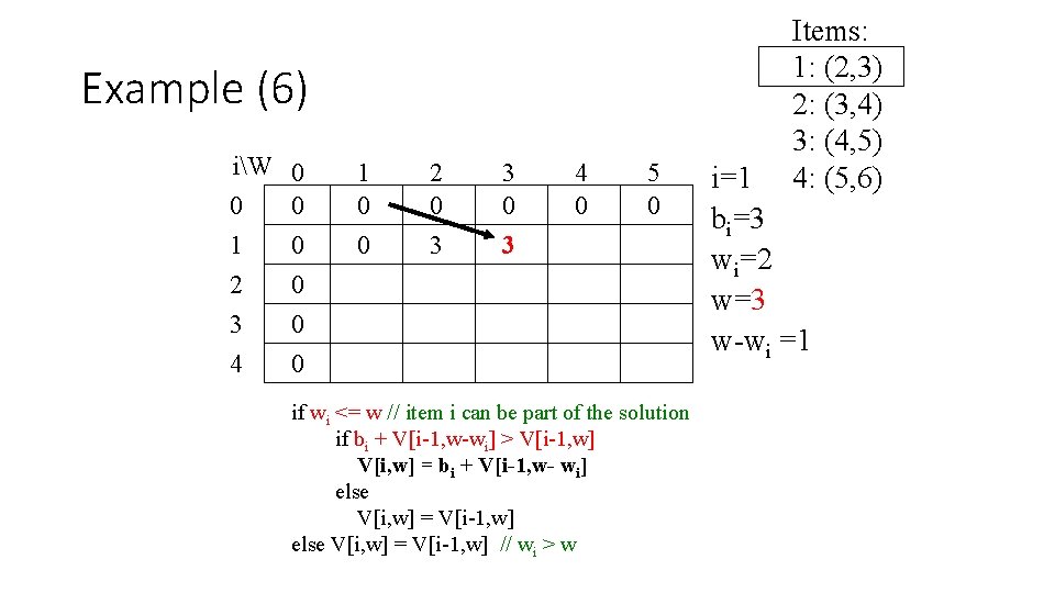
Example (6) iW 0 0 0 1 0 2 0 3 0 4 0 1 0 0 2 0 3 3 0 3 4 0 5 0 if wi <= w // item i can be part of the solution if bi + V[i-1, w-wi] > V[i-1, w] V[i, w] = bi + V[i-1, w- wi] else V[i, w] = V[i-1, w] // wi > w Items: 1: (2, 3) 2: (3, 4) 3: (4, 5) 4: (5, 6) i=1 bi=3 wi=2 w=3 w-wi =1

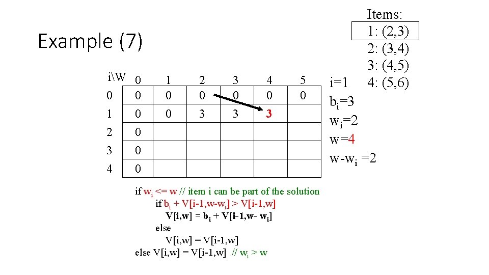
Example (7) iW 0 0 0 1 0 2 0 3 0 4 0 1 0 0 2 0 3 3 0 3 4 0 3 5 0 if wi <= w // item i can be part of the solution if bi + V[i-1, w-wi] > V[i-1, w] V[i, w] = bi + V[i-1, w- wi] else V[i, w] = V[i-1, w] // wi > w Items: 1: (2, 3) 2: (3, 4) 3: (4, 5) 4: (5, 6) i=1 bi=3 wi=2 w=4 w-wi =2

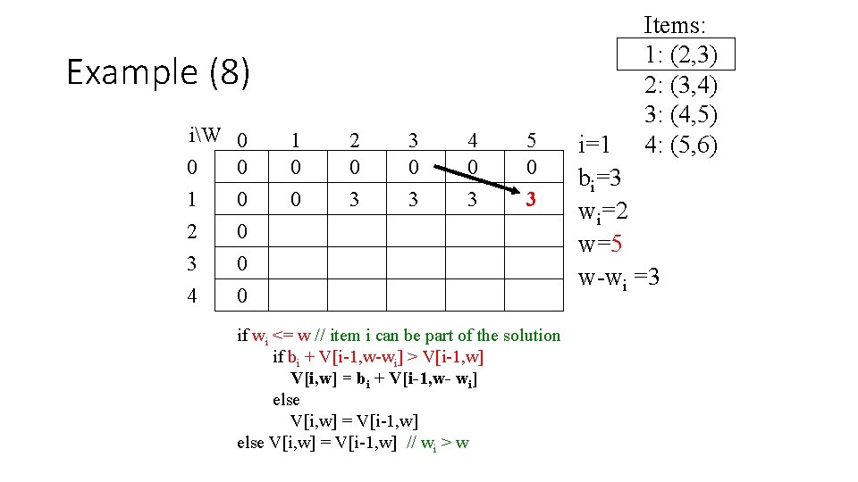
Example (8) iW 0 0 0 1 0 2 0 3 0 4 0 1 0 0 2 0 3 3 0 3 4 0 3 5 0 3 if wi <= w // item i can be part of the solution if bi + V[i-1, w-wi] > V[i-1, w] V[i, w] = bi + V[i-1, w- wi] else V[i, w] = V[i-1, w] // wi > w Items: 1: (2, 3) 2: (3, 4) 3: (4, 5) 4: (5, 6) i=1 bi=3 wi=2 w=5 w-wi =3

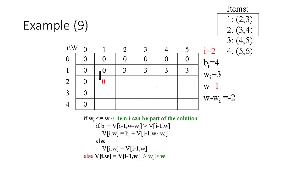
Example (9) iW 0 0 0 1 0 2 0 3 0 4 0 1 0 0 0 2 0 3 3 0 3 4 0 3 5 0 3 if wi <= w // item i can be part of the solution if bi + V[i-1, w-wi] > V[i-1, w] V[i, w] = bi + V[i-1, w- wi] else V[i, w] = V[i-1, w] // wi > w Items: 1: (2, 3) 2: (3, 4) 3: (4, 5) 4: (5, 6) i=2 bi=4 wi=3 w=1 w-wi =-2

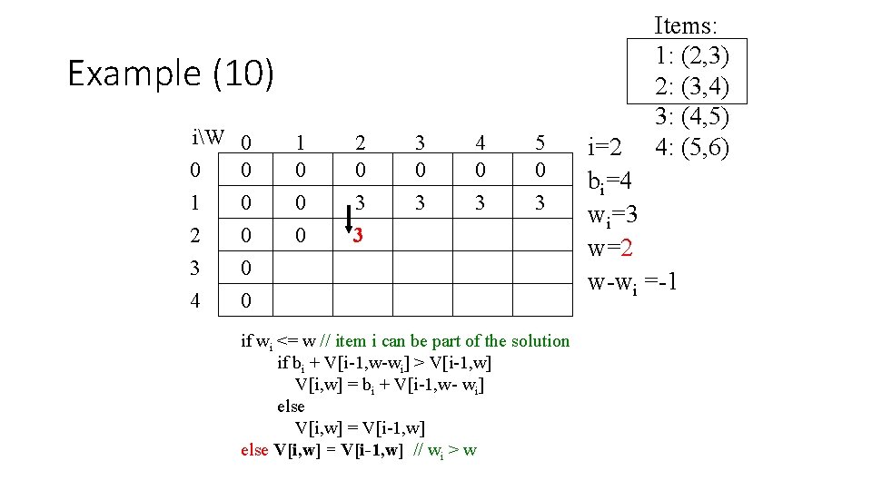
Example (10) iW 0 0 0 1 0 2 0 3 0 4 0 1 0 0 0 2 0 3 3 3 0 3 4 0 3 5 0 3 if wi <= w // item i can be part of the solution if bi + V[i-1, w-wi] > V[i-1, w] V[i, w] = bi + V[i-1, w- wi] else V[i, w] = V[i-1, w] // wi > w Items: 1: (2, 3) 2: (3, 4) 3: (4, 5) 4: (5, 6) i=2 bi=4 wi=3 w=2 w-wi =-1

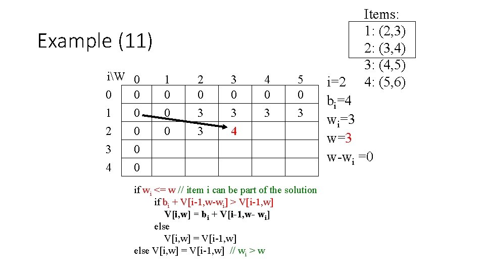
Example (11) iW 0 0 0 1 0 2 0 3 0 4 0 1 0 0 0 2 0 3 3 3 0 3 4 4 0 3 5 0 3 if wi <= w // item i can be part of the solution if bi + V[i-1, w-wi] > V[i-1, w] V[i, w] = bi + V[i-1, w- wi] else V[i, w] = V[i-1, w] // wi > w Items: 1: (2, 3) 2: (3, 4) 3: (4, 5) 4: (5, 6) i=2 bi=4 wi=3 w-wi =0

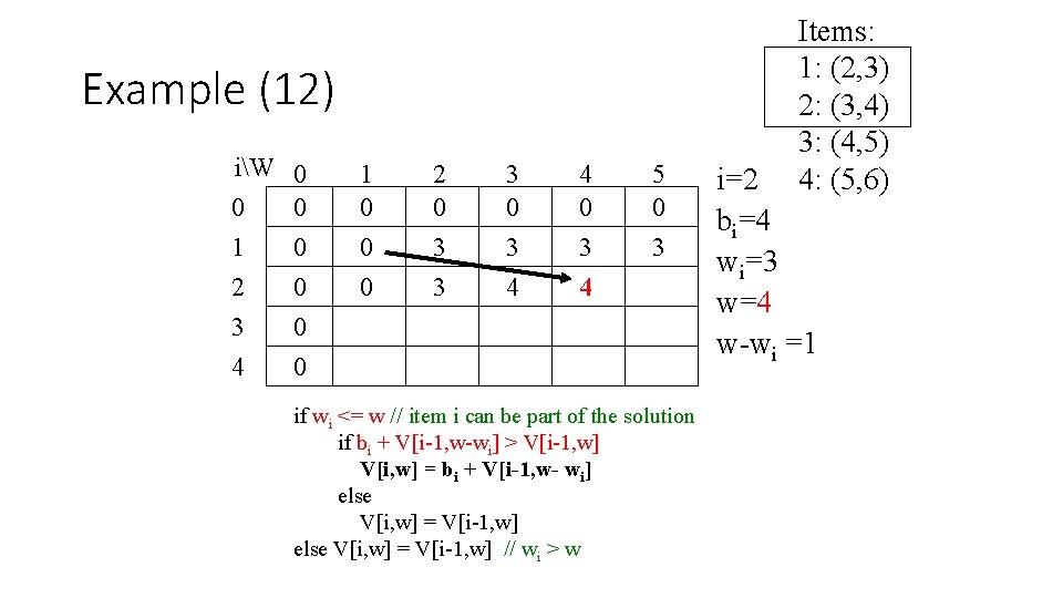
Example (12) iW 0 0 0 1 0 2 0 3 0 4 0 1 0 0 0 2 0 3 3 3 0 3 4 4 0 3 4 5 0 3 if wi <= w // item i can be part of the solution if bi + V[i-1, w-wi] > V[i-1, w] V[i, w] = bi + V[i-1, w- wi] else V[i, w] = V[i-1, w] // wi > w Items: 1: (2, 3) 2: (3, 4) 3: (4, 5) 4: (5, 6) i=2 bi=4 wi=3 w=4 w-wi =1

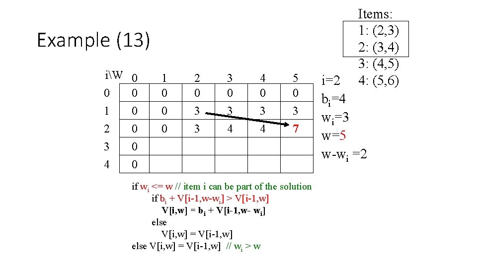
Example (13) iW 0 0 0 1 0 2 0 3 0 4 0 1 0 0 0 2 0 3 3 3 0 3 4 4 0 3 4 5 0 3 7 if wi <= w // item i can be part of the solution if bi + V[i-1, w-wi] > V[i-1, w] V[i, w] = bi + V[i-1, w- wi] else V[i, w] = V[i-1, w] // wi > w Items: 1: (2, 3) 2: (3, 4) 3: (4, 5) 4: (5, 6) i=2 bi=4 wi=3 w=5 w-wi =2

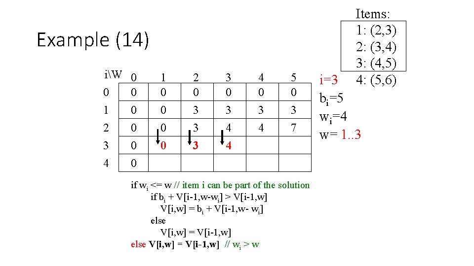
Example (14) iW 0 0 0 1 0 2 0 3 0 4 0 1 0 0 2 0 3 3 0 3 4 4 4 0 3 4 5 0 3 7 if wi <= w // item i can be part of the solution if bi + V[i-1, w-wi] > V[i-1, w] V[i, w] = bi + V[i-1, w- wi] else V[i, w] = V[i-1, w] // wi > w Items: 1: (2, 3) 2: (3, 4) 3: (4, 5) 4: (5, 6) i=3 bi=5 wi=4 w= 1. . 3

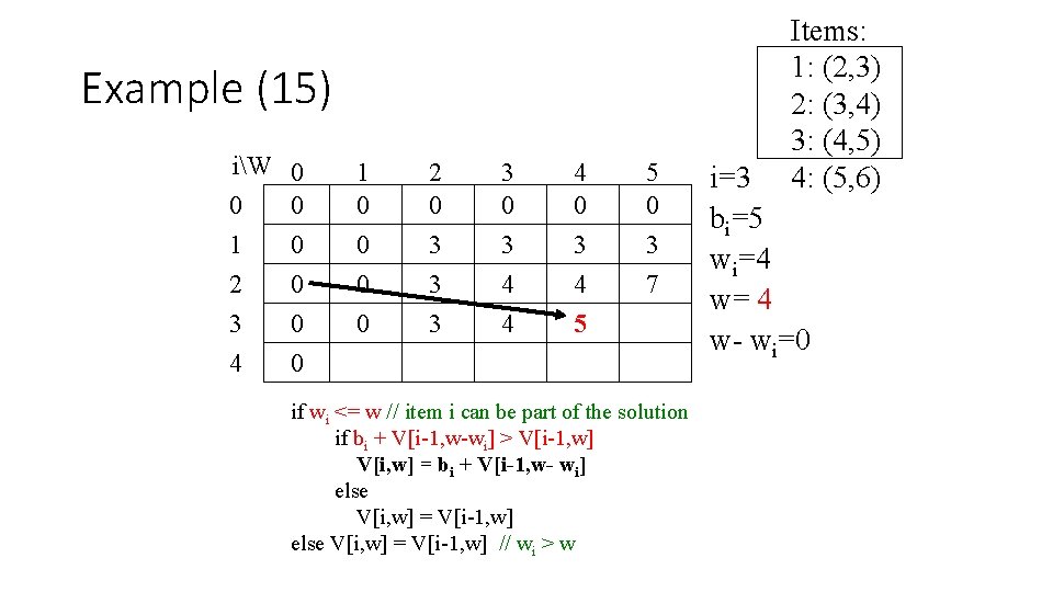
Example (15) iW 0 0 0 1 0 2 0 3 0 4 0 1 0 0 2 0 3 3 0 3 4 4 4 0 3 4 5 5 0 3 7 if wi <= w // item i can be part of the solution if bi + V[i-1, w-wi] > V[i-1, w] V[i, w] = bi + V[i-1, w- wi] else V[i, w] = V[i-1, w] // wi > w Items: 1: (2, 3) 2: (3, 4) 3: (4, 5) 4: (5, 6) i=3 bi=5 wi=4 w= 4 w- wi=0

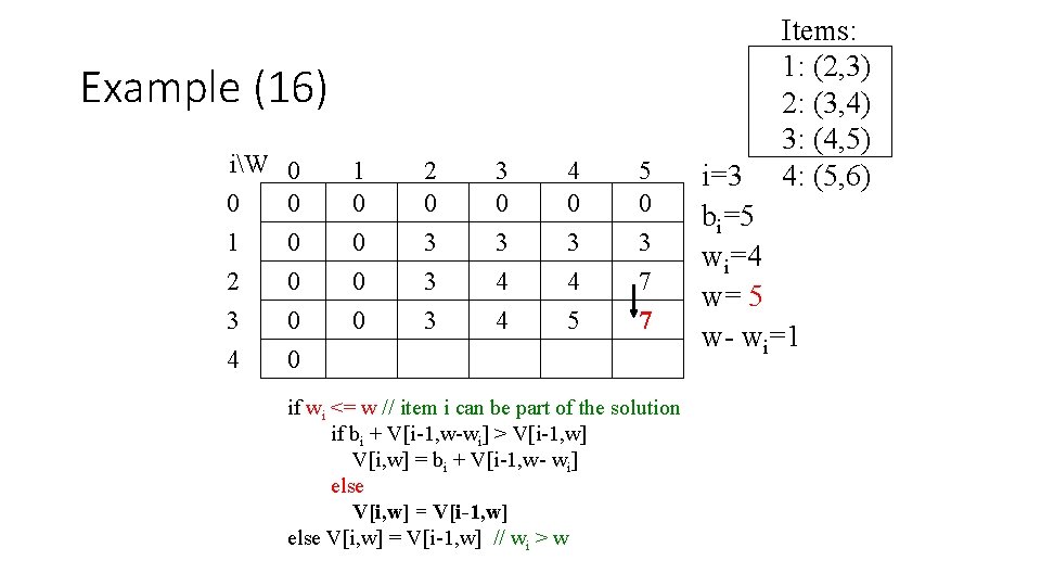
Example (16) iW 0 0 0 1 0 2 0 3 0 4 0 1 0 0 2 0 3 3 0 3 4 4 4 0 3 4 5 5 0 3 7 7 if wi <= w // item i can be part of the solution if bi + V[i-1, w-wi] > V[i-1, w] V[i, w] = bi + V[i-1, w- wi] else V[i, w] = V[i-1, w] // wi > w Items: 1: (2, 3) 2: (3, 4) 3: (4, 5) 4: (5, 6) i=3 bi=5 wi=4 w= 5 w- wi=1

Example (17) iW 0 0 0 1 0 2 0 3 0 4 0 1 0 0 0 2 0 3 3 3 0 3 4 4 0 3 4 5 5 5 0 3 7 7 if wi <= w // item i can be part of the solution if bi + V[i-1, w-wi] > V[i-1, w] V[i, w] = bi + V[i-1, w- wi] else V[i, w] = V[i-1, w] // wi > w Items: 1: (2, 3) 2: (3, 4) 3: (4, 5) 4: (5, 6) i=4 bi=6 wi=5 w= 1. . 4

Example (18) iW 0 0 0 1 0 2 0 3 0 4 0 1 0 0 0 2 0 3 3 3 0 3 4 4 0 3 4 5 5 5 0 3 7 7 7 if wi <= w // item i can be part of the solution if bi + V[i-1, w-wi] > V[i-1, w] V[i, w] = bi + V[i-1, w- wi] else V[i, w] = V[i-1, w] // wi > w Items: 1: (2, 3) 2: (3, 4) 3: (4, 5) 4: (5, 6) i=4 bi=6 wi=5 w= 5 w- wi=0
![0 1 Knapsack Memory Function Algorithm MFKnapsacki W if Vi W 0 if 0 -1 Knapsack Memory Function Algorithm MFKnapsack(i, W) if V[i, W] < 0 if](https://slidetodoc.com/presentation_image_h2/8c64bd176572e15b90d7fc2a71c9293c/image-42.jpg)
0 -1 Knapsack Memory Function Algorithm MFKnapsack(i, W) if V[i, W] < 0 if W < wi value = MFKnapsack(i-1, W) else value = max(MFKnapsack(i-1, W), vi + MFKnapsack(i-1, W-wi)) V[i, W] = value return V[i, W]

S=Φ Cost(2, Φ, 1)=d(2, 1)=5 Cost(3, Φ, 1)=d(3, 1)=6 Cost(4, Φ, 1)=d(4, 1)=8 S
