Dynamic Programming Dynamic Programming Dynamic programming like the

Dynamic Programming

Dynamic Programming • Dynamic programming, like the divide-and-conquer method, solves problems by combining the solutions to sub-problems. • “Programming” in this context refers to a tabular method, not to writing computer code. • We typically apply dynamic programming to optimization problems • Many possible solutions. Each solution has a value, and we wish to find a solution with the optimal (minimum or maximum) value.

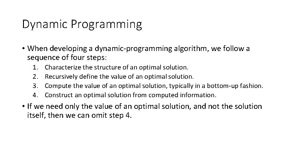
Dynamic Programming • When developing a dynamic-programming algorithm, we follow a sequence of four steps: 1. 2. 3. 4. Characterize the structure of an optimal solution. Recursively define the value of an optimal solution. Compute the value of an optimal solution, typically in a bottom-up fashion. Construct an optimal solution from computed information. • If we need only the value of an optimal solution, and not the solution itself, then we can omit step 4.

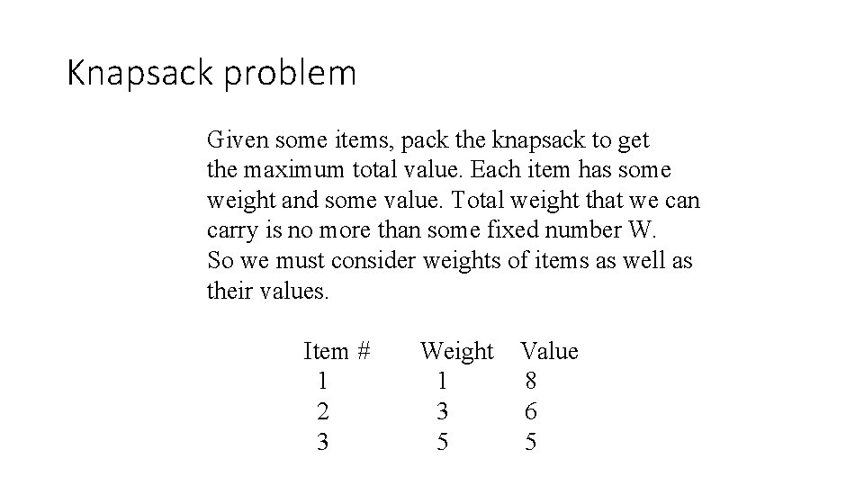
Knapsack problem Given some items, pack the knapsack to get the maximum total value. Each item has some weight and some value. Total weight that we can carry is no more than some fixed number W. So we must consider weights of items as well as their values. Item # 1 2 3 Weight 1 3 5 Value 8 6 5

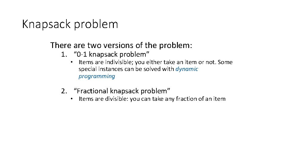
Knapsack problem There are two versions of the problem: 1. “ 0 -1 knapsack problem” • Items are indivisible; you either take an item or not. Some special instances can be solved with dynamic programming 2. “Fractional knapsack problem” • Items are divisible: you can take any fraction of an item

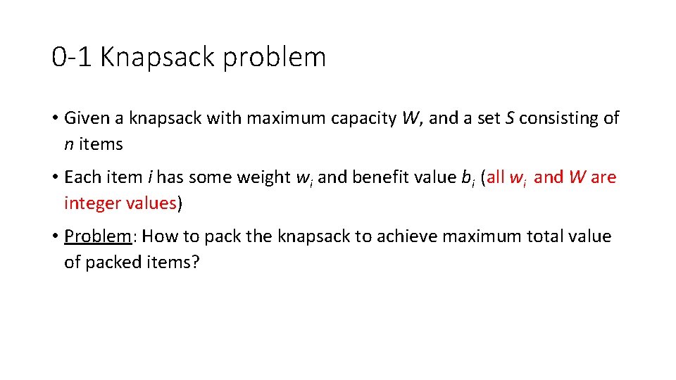
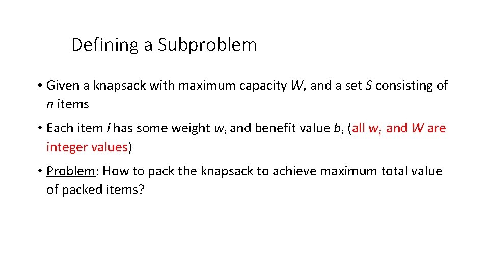
0 -1 Knapsack problem • Given a knapsack with maximum capacity W, and a set S consisting of n items • Each item i has some weight wi and benefit value bi (all wi and W are integer values) • Problem: How to pack the knapsack to achieve maximum total value of packed items?

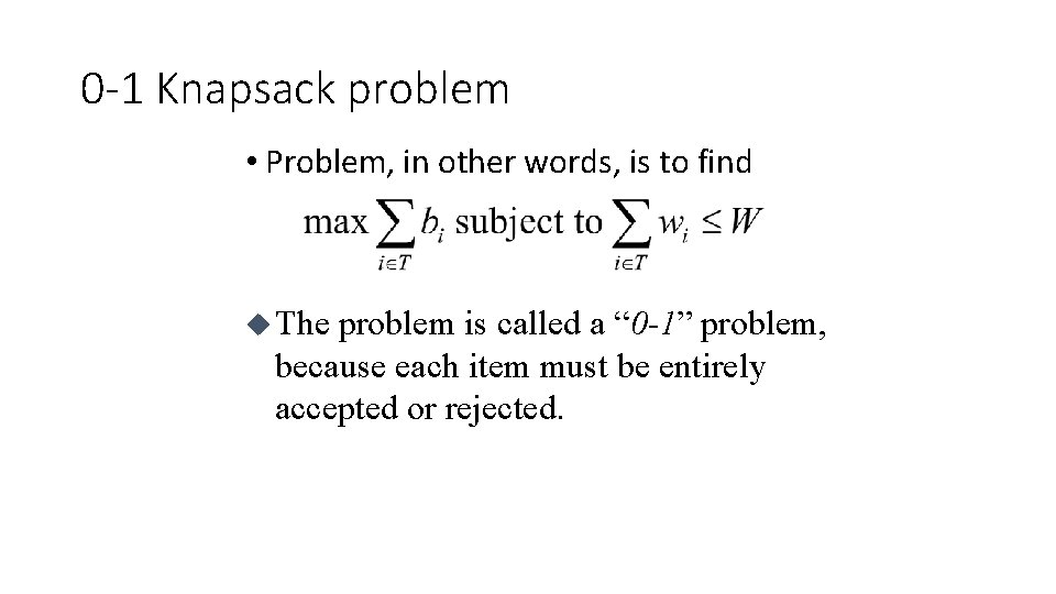
0 -1 Knapsack problem • Problem, in other words, is to find u The problem is called a “ 0 -1” problem, because each item must be entirely accepted or rejected.

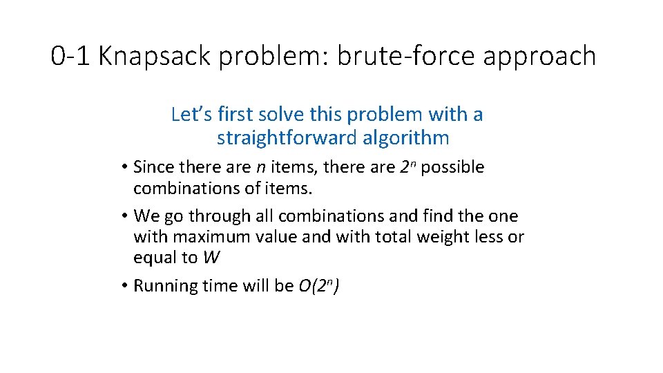
0 -1 Knapsack problem: brute-force approach Let’s first solve this problem with a straightforward algorithm • Since there are n items, there are 2 n possible combinations of items. • We go through all combinations and find the one with maximum value and with total weight less or equal to W • Running time will be O(2 n)

0 -1 Knapsack problem: dynamic programming approach • We can do better with an algorithm based on dynamic programming • We need to carefully identify the subproblems

Defining a Subproblem • Given a knapsack with maximum capacity W, and a set S consisting of n items • Each item i has some weight wi and benefit value bi (all wi and W are integer values) • Problem: How to pack the knapsack to achieve maximum total value of packed items?

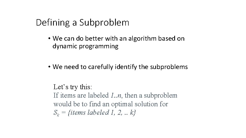
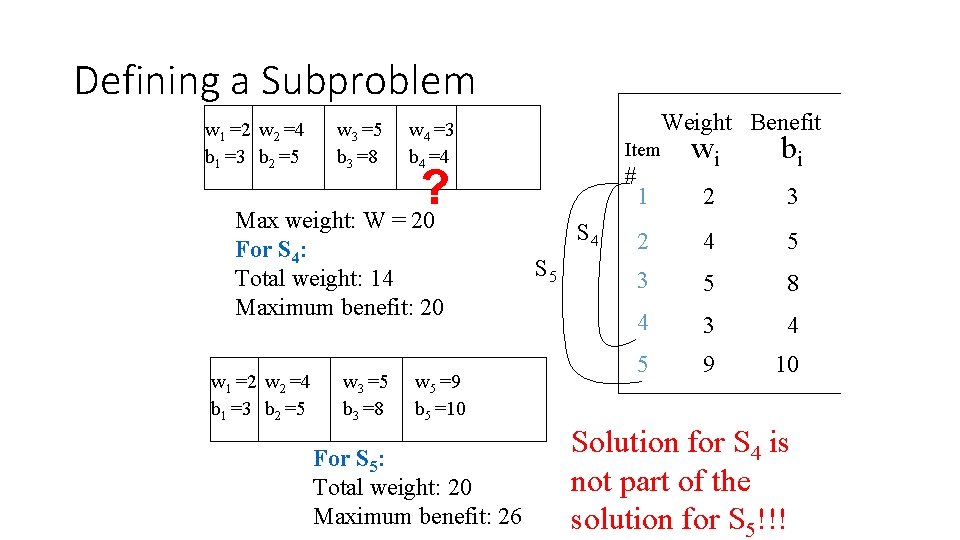
Defining a Subproblem • We can do better with an algorithm based on dynamic programming • We need to carefully identify the subproblems Let’s try this: If items are labeled 1. . n, then a subproblem would be to find an optimal solution for Sk = {items labeled 1, 2, . . k}

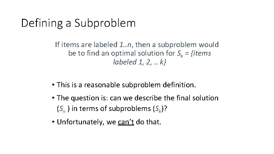
Defining a Subproblem If items are labeled 1. . n, then a subproblem would be to find an optimal solution for Sk = {items labeled 1, 2, . . k} • This is a reasonable subproblem definition. • The question is: can we describe the final solution (Sn ) in terms of subproblems (Sk)? • Unfortunately, we can’t do that.

Defining a Subproblem w 1 =2 w 2 =4 b 1 =3 b 2 =5 w 3 =5 b 3 =8 w 5 =9 b 5 =10 For S 5: Total weight: 20 Maximum benefit: 26 wi bi 1 2 3 2 4 5 3 5 8 4 3 4 5 9 10 Item ? Max weight: W = 20 For S 4: Total weight: 14 Maximum benefit: 20 w 1 =2 w 2 =4 b 1 =3 b 2 =5 Weight Benefit w 4 =3 b 4 =4 # S 4 S 5 Solution for S 4 is not part of the solution for S 5!!!

Defining a Subproblem • As we have seen, the solution for S 4 is not part of the solution for S 5 • So our definition of a subproblem is flawed and we need another one!

Defining a Subproblem • Given a knapsack with maximum capacity W, and a set S consisting of n items • Each item i has some weight wi and benefit value bi (all wi and W are integer values) • Problem: How to pack the knapsack to achieve maximum total value of packed items?

Defining a Subproblem • Let’s add another parameter: w, which will represent the maximum weight for each subset of items • The subproblem then will be to compute V[k, w], i. e. , to find an optimal solution for Sk = {items labeled 1, 2, . . k} in a knapsack of size w

Recursive Formula for subproblems • The subproblem will then be to compute V[k, w], i. e. , to find an optimal solution for Sk = {items labeled 1, 2, . . k} in a knapsack of size w • Assuming knowing V[i, j], where i=0, 1, 2, … k-1, j=0, 1, 2, …w, how to derive V[k, w]?

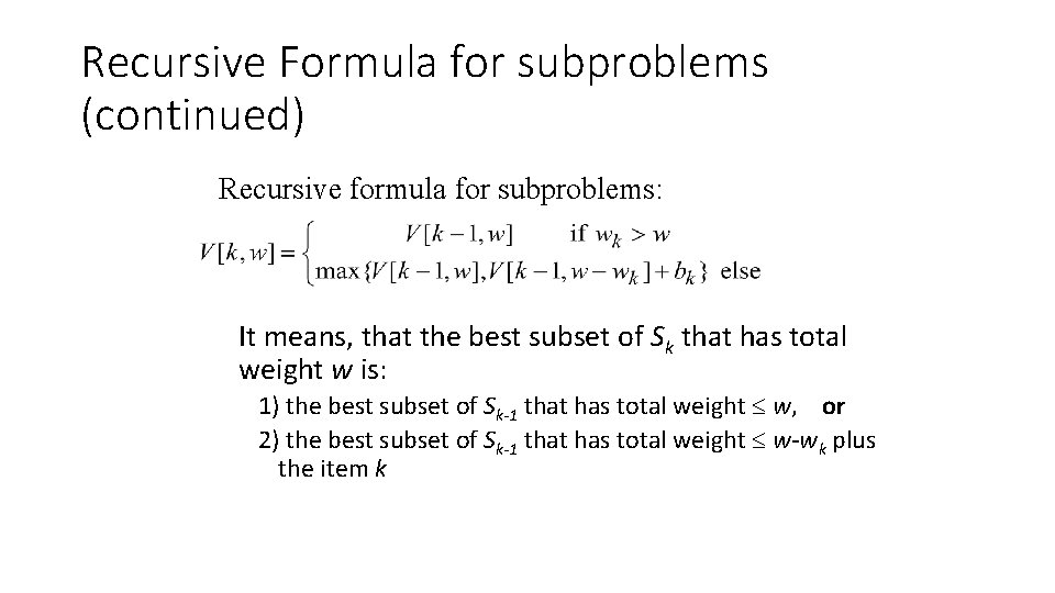
Recursive Formula for subproblems (continued) Recursive formula for subproblems: It means, that the best subset of Sk that has total weight w is: 1) the best subset of Sk-1 that has total weight w, or 2) the best subset of Sk-1 that has total weight w-wk plus the item k

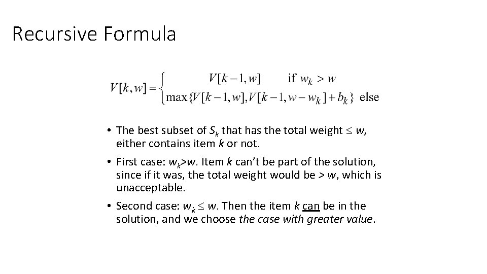
Recursive Formula • The best subset of Sk that has the total weight w, either contains item k or not. • First case: wk>w. Item k can’t be part of the solution, since if it was, the total weight would be > w, which is unacceptable. • Second case: wk w. Then the item k can be in the solution, and we choose the case with greater value.

0 -1 Knapsack Algorithm for w = 0 to W V[0, w] = 0 for i = 1 to n V[i, 0] = 0 for i = 1 to n for w = 0 to W if wi <= w // item i can be part of the solution if bi + V[i-1, w-wi] > V[i-1, w] V[i, w] = bi + V[i-1, w- wi] else V[i, w] = V[i-1, w] // wi > w

Running time for w = 0 to W O(W) V[0, w] = 0 for i = 1 to n V[i, 0] = 0 for i = 1 to n Repeat n for w = 0 to W < the rest of the code O(W) > times What is the running time of this algorithm? O(n*W) Remember that the brute-force algorithm takes O(2 n)

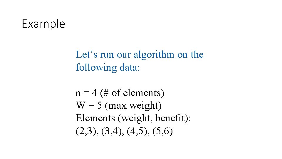
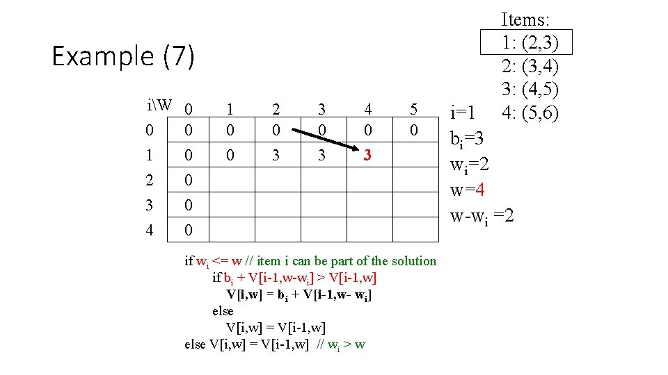
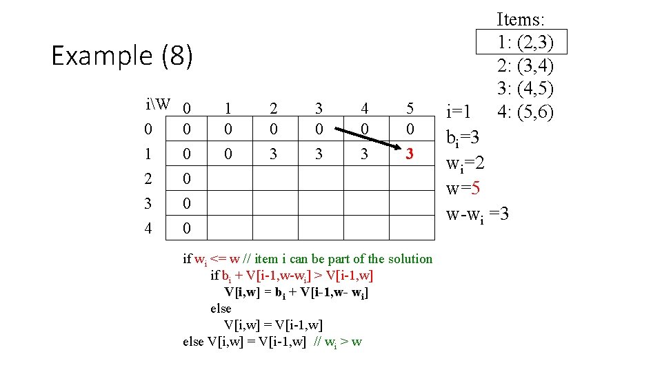
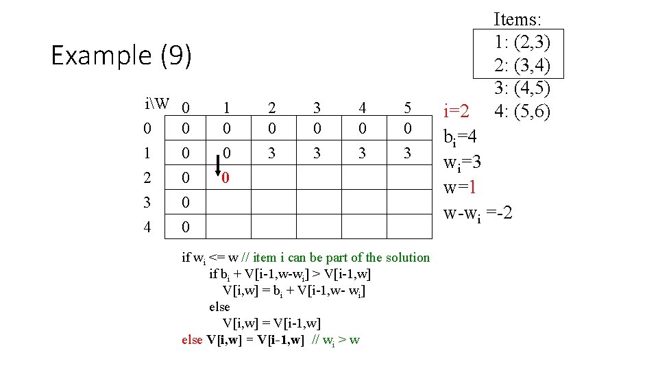
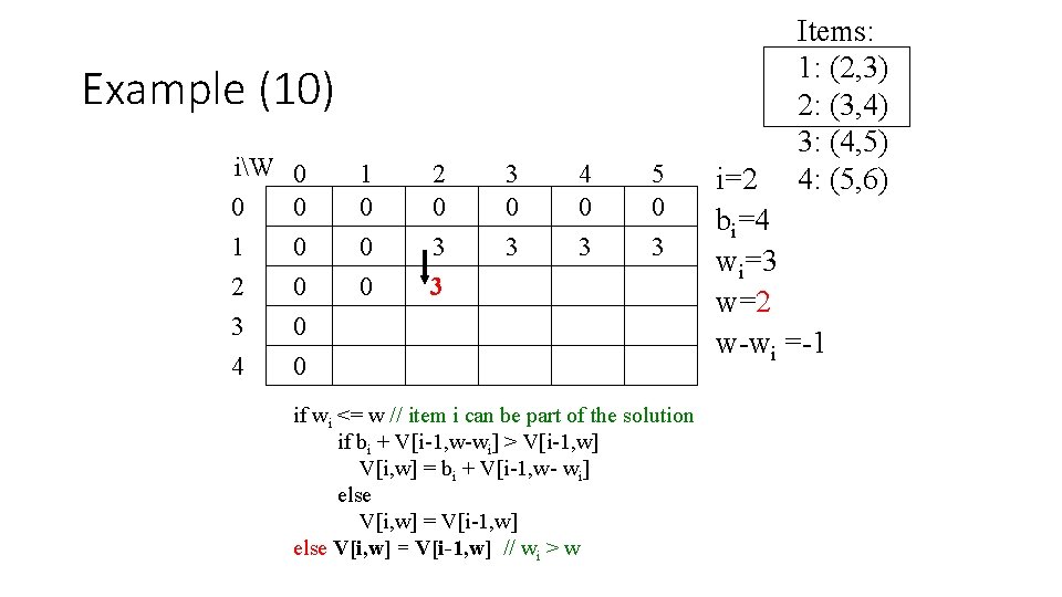
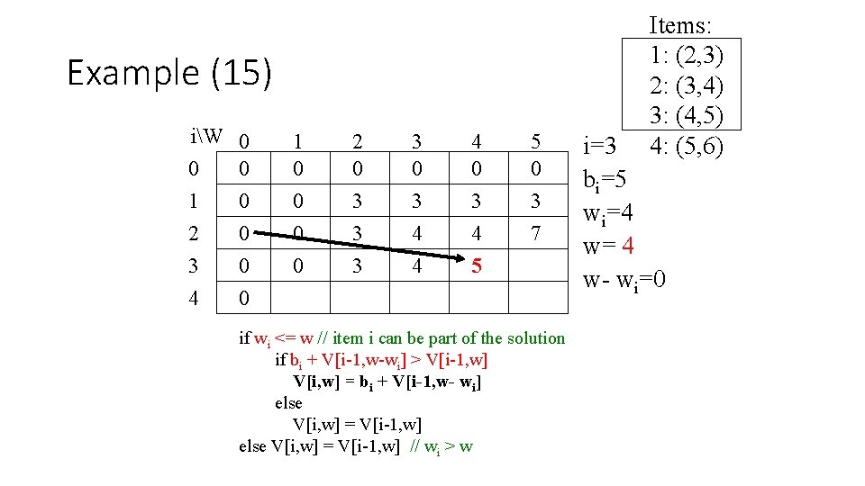
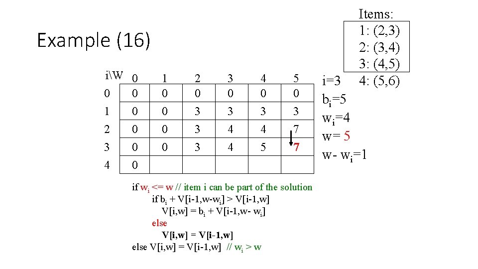
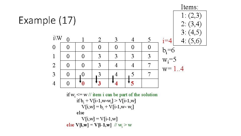
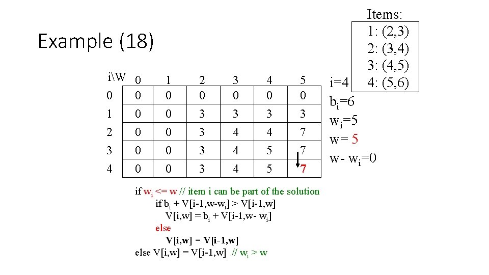
Example Let’s run our algorithm on the following data: n = 4 (# of elements) W = 5 (max weight) Elements (weight, benefit): (2, 3), (3, 4), (4, 5), (5, 6)

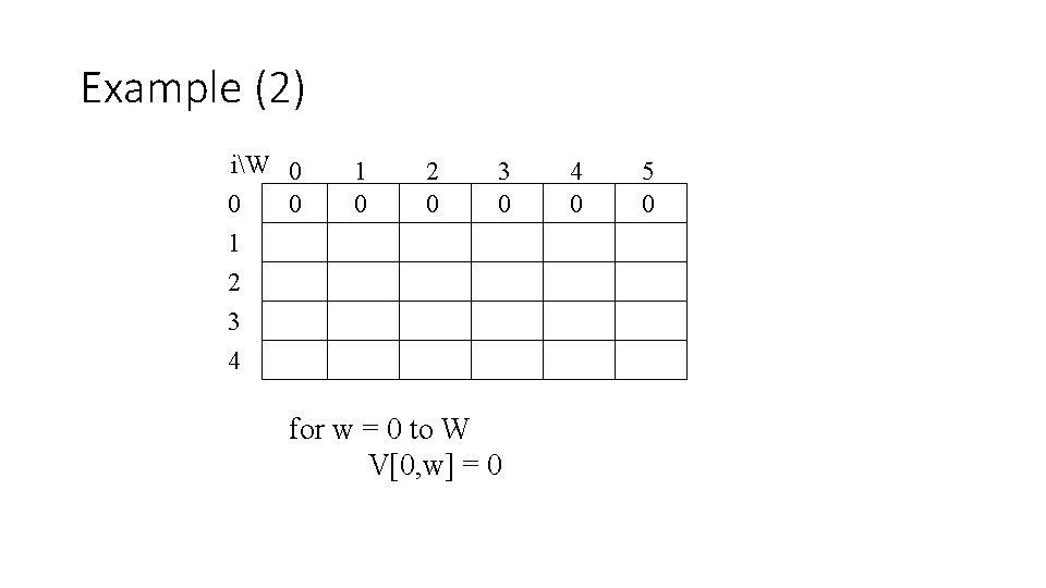
Example (2) iW 0 0 0 1 2 3 4 1 0 2 0 3 0 for w = 0 to W V[0, w] = 0 4 0 5 0

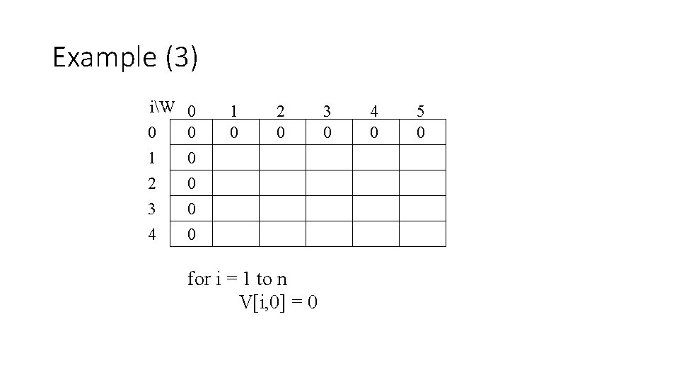
Example (3) iW 0 1 2 3 4 0 0 0 1 0 2 0 for i = 1 to n V[i, 0] = 0 3 0 4 0 5 0

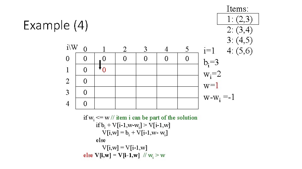
Example (4) iW 0 1 2 3 4 0 0 0 1 0 0 2 0 3 0 4 0 5 0 if wi <= w // item i can be part of the solution if bi + V[i-1, w-wi] > V[i-1, w] V[i, w] = bi + V[i-1, w- wi] else V[i, w] = V[i-1, w] // wi > w Items: 1: (2, 3) 2: (3, 4) 3: (4, 5) 4: (5, 6) i=1 bi=3 wi=2 w=1 w-wi =-1

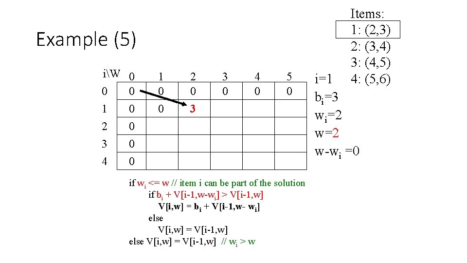
Example (5) iW 0 0 0 1 0 2 0 3 0 4 0 1 0 0 2 0 3 3 0 4 0 5 0 if wi <= w // item i can be part of the solution if bi + V[i-1, w-wi] > V[i-1, w] V[i, w] = bi + V[i-1, w- wi] else V[i, w] = V[i-1, w] // wi > w Items: 1: (2, 3) 2: (3, 4) 3: (4, 5) 4: (5, 6) i=1 bi=3 wi=2 w-wi =0

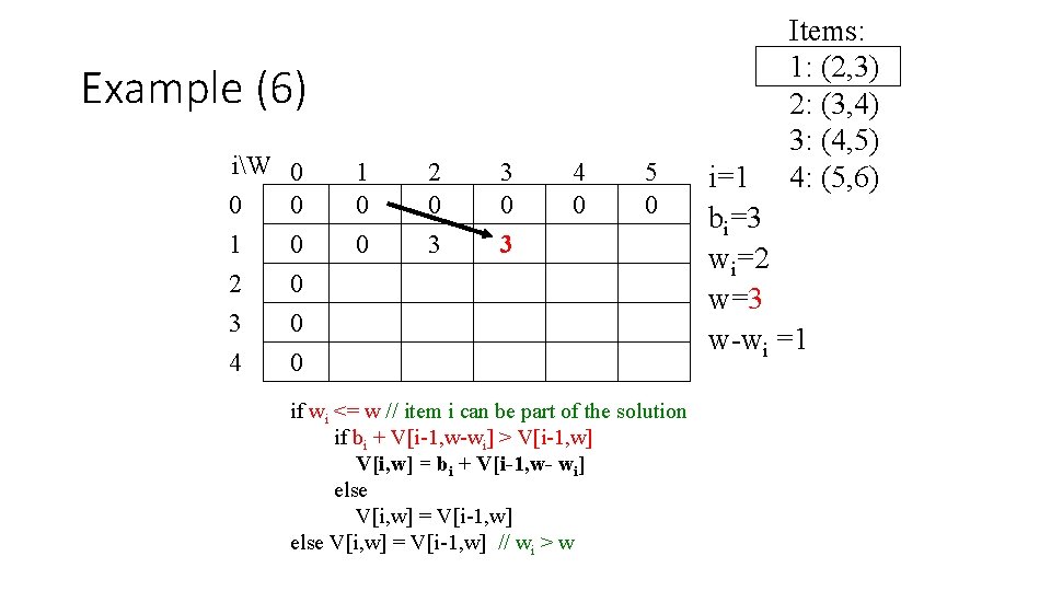
Example (6) iW 0 0 0 1 0 2 0 3 0 4 0 1 0 0 2 0 3 3 0 3 4 0 5 0 if wi <= w // item i can be part of the solution if bi + V[i-1, w-wi] > V[i-1, w] V[i, w] = bi + V[i-1, w- wi] else V[i, w] = V[i-1, w] // wi > w Items: 1: (2, 3) 2: (3, 4) 3: (4, 5) 4: (5, 6) i=1 bi=3 wi=2 w=3 w-wi =1

Example (7) iW 0 0 0 1 0 2 0 3 0 4 0 1 0 0 2 0 3 3 0 3 4 0 3 5 0 if wi <= w // item i can be part of the solution if bi + V[i-1, w-wi] > V[i-1, w] V[i, w] = bi + V[i-1, w- wi] else V[i, w] = V[i-1, w] // wi > w Items: 1: (2, 3) 2: (3, 4) 3: (4, 5) 4: (5, 6) i=1 bi=3 wi=2 w=4 w-wi =2

Example (8) iW 0 0 0 1 0 2 0 3 0 4 0 1 0 0 2 0 3 3 0 3 4 0 3 5 0 3 if wi <= w // item i can be part of the solution if bi + V[i-1, w-wi] > V[i-1, w] V[i, w] = bi + V[i-1, w- wi] else V[i, w] = V[i-1, w] // wi > w Items: 1: (2, 3) 2: (3, 4) 3: (4, 5) 4: (5, 6) i=1 bi=3 wi=2 w=5 w-wi =3

Example (9) iW 0 0 0 1 0 2 0 3 0 4 0 1 0 0 0 2 0 3 3 0 3 4 0 3 5 0 3 if wi <= w // item i can be part of the solution if bi + V[i-1, w-wi] > V[i-1, w] V[i, w] = bi + V[i-1, w- wi] else V[i, w] = V[i-1, w] // wi > w Items: 1: (2, 3) 2: (3, 4) 3: (4, 5) 4: (5, 6) i=2 bi=4 wi=3 w=1 w-wi =-2

Example (10) iW 0 0 0 1 0 2 0 3 0 4 0 1 0 0 0 2 0 3 3 3 0 3 4 0 3 5 0 3 if wi <= w // item i can be part of the solution if bi + V[i-1, w-wi] > V[i-1, w] V[i, w] = bi + V[i-1, w- wi] else V[i, w] = V[i-1, w] // wi > w Items: 1: (2, 3) 2: (3, 4) 3: (4, 5) 4: (5, 6) i=2 bi=4 wi=3 w=2 w-wi =-1

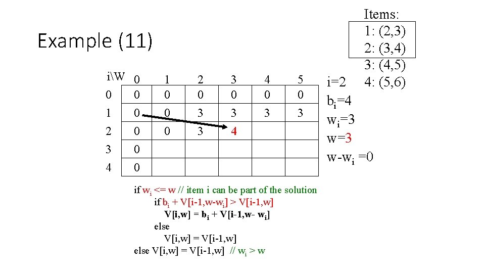
Example (11) iW 0 0 0 1 0 2 0 3 0 4 0 1 0 0 0 2 0 3 3 3 0 3 4 4 0 3 5 0 3 if wi <= w // item i can be part of the solution if bi + V[i-1, w-wi] > V[i-1, w] V[i, w] = bi + V[i-1, w- wi] else V[i, w] = V[i-1, w] // wi > w Items: 1: (2, 3) 2: (3, 4) 3: (4, 5) 4: (5, 6) i=2 bi=4 wi=3 w-wi =0

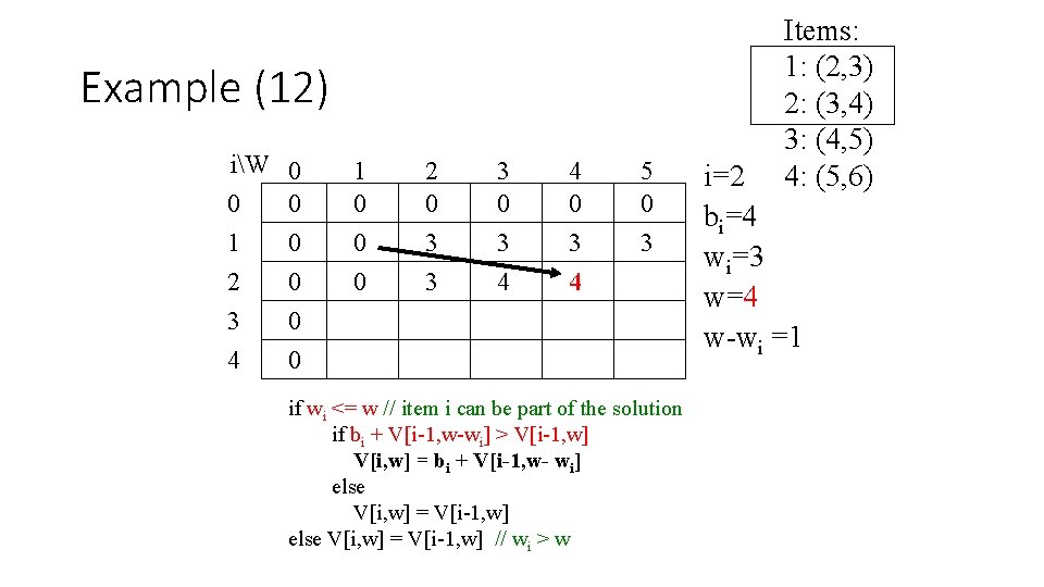
Example (12) iW 0 0 0 1 0 2 0 3 0 4 0 1 0 0 0 2 0 3 3 3 0 3 4 4 0 3 4 5 0 3 if wi <= w // item i can be part of the solution if bi + V[i-1, w-wi] > V[i-1, w] V[i, w] = bi + V[i-1, w- wi] else V[i, w] = V[i-1, w] // wi > w Items: 1: (2, 3) 2: (3, 4) 3: (4, 5) 4: (5, 6) i=2 bi=4 wi=3 w=4 w-wi =1

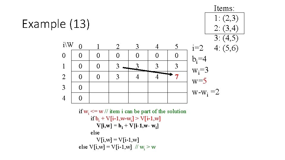
Example (13) iW 0 0 0 1 0 2 0 3 0 4 0 1 0 0 0 2 0 3 3 3 0 3 4 4 0 3 4 5 0 3 7 if wi <= w // item i can be part of the solution if bi + V[i-1, w-wi] > V[i-1, w] V[i, w] = bi + V[i-1, w- wi] else V[i, w] = V[i-1, w] // wi > w Items: 1: (2, 3) 2: (3, 4) 3: (4, 5) 4: (5, 6) i=2 bi=4 wi=3 w=5 w-wi =2

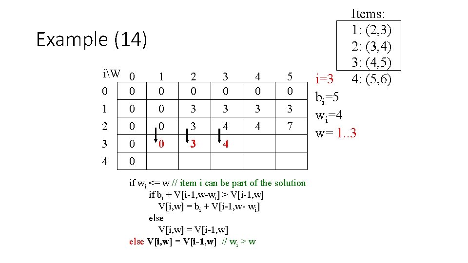
Example (14) iW 0 0 0 1 0 2 0 3 0 4 0 1 0 0 2 0 3 3 0 3 4 4 4 0 3 4 5 0 3 7 if wi <= w // item i can be part of the solution if bi + V[i-1, w-wi] > V[i-1, w] V[i, w] = bi + V[i-1, w- wi] else V[i, w] = V[i-1, w] // wi > w Items: 1: (2, 3) 2: (3, 4) 3: (4, 5) 4: (5, 6) i=3 bi=5 wi=4 w= 1. . 3

Example (15) iW 0 0 0 1 0 2 0 3 0 4 0 1 0 0 2 0 3 3 0 3 4 4 4 0 3 4 5 5 0 3 7 if wi <= w // item i can be part of the solution if bi + V[i-1, w-wi] > V[i-1, w] V[i, w] = bi + V[i-1, w- wi] else V[i, w] = V[i-1, w] // wi > w Items: 1: (2, 3) 2: (3, 4) 3: (4, 5) 4: (5, 6) i=3 bi=5 wi=4 w= 4 w- wi=0

Example (16) iW 0 0 0 1 0 2 0 3 0 4 0 1 0 0 2 0 3 3 0 3 4 4 4 0 3 4 5 5 0 3 7 7 if wi <= w // item i can be part of the solution if bi + V[i-1, w-wi] > V[i-1, w] V[i, w] = bi + V[i-1, w- wi] else V[i, w] = V[i-1, w] // wi > w Items: 1: (2, 3) 2: (3, 4) 3: (4, 5) 4: (5, 6) i=3 bi=5 wi=4 w= 5 w- wi=1

Example (17) iW 0 0 0 1 0 2 0 3 0 4 0 1 0 0 0 2 0 3 3 3 0 3 4 4 0 3 4 5 5 5 0 3 7 7 if wi <= w // item i can be part of the solution if bi + V[i-1, w-wi] > V[i-1, w] V[i, w] = bi + V[i-1, w- wi] else V[i, w] = V[i-1, w] // wi > w Items: 1: (2, 3) 2: (3, 4) 3: (4, 5) 4: (5, 6) i=4 bi=6 wi=5 w= 1. . 4

Example (18) iW 0 0 0 1 0 2 0 3 0 4 0 1 0 0 0 2 0 3 3 3 0 3 4 4 0 3 4 5 5 5 0 3 7 7 7 if wi <= w // item i can be part of the solution if bi + V[i-1, w-wi] > V[i-1, w] V[i, w] = bi + V[i-1, w- wi] else V[i, w] = V[i-1, w] // wi > w Items: 1: (2, 3) 2: (3, 4) 3: (4, 5) 4: (5, 6) i=4 bi=6 wi=5 w= 5 w- wi=0

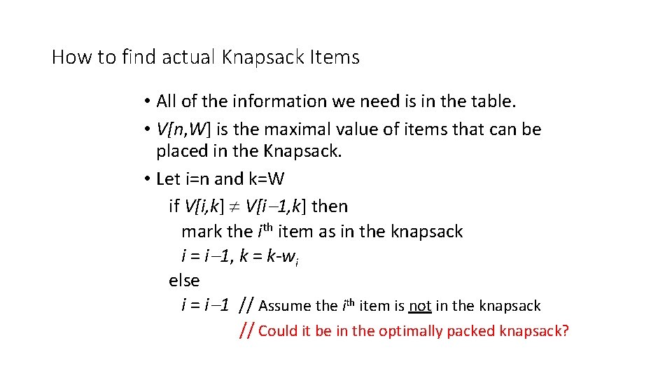
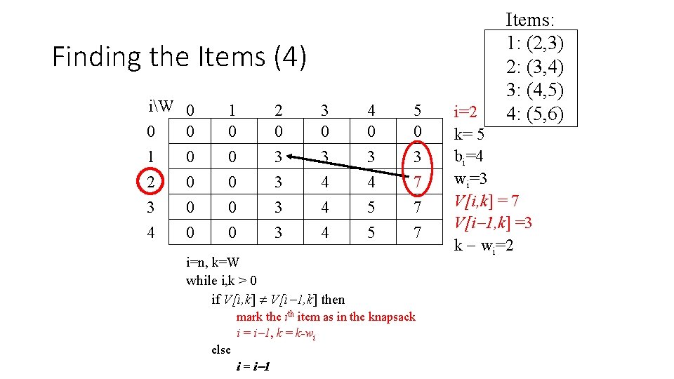
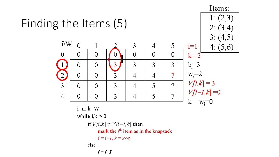
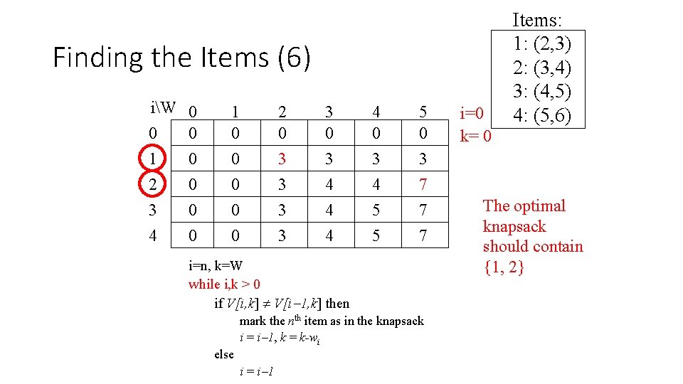
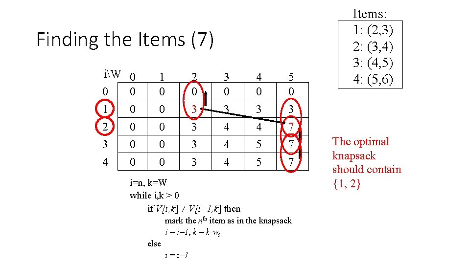
How to find actual Knapsack Items • All of the information we need is in the table. • V[n, W] is the maximal value of items that can be placed in the Knapsack. • Let i=n and k=W if V[i, k] V[i 1, k] then mark the ith item as in the knapsack i = i 1, k = k-wi else i = i 1 // Assume the ith item is not in the knapsack // Could it be in the optimally packed knapsack?

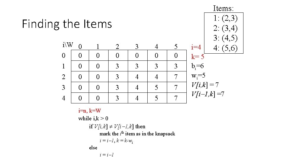
Finding the Items iW 0 0 0 1 0 2 0 3 0 4 0 1 0 0 0 2 0 3 3 3 0 3 4 4 0 3 4 5 5 5 0 3 7 7 7 i=n, k=W while i, k > 0 if V[i, k] V[i 1, k] then mark the ith item as in the knapsack i = i 1, k = k-wi else i = i 1 Items: 1: (2, 3) 2: (3, 4) 3: (4, 5) 4: (5, 6) i=4 k= 5 bi=6 wi=5 V[i, k] = 7 V[i 1, k] =7

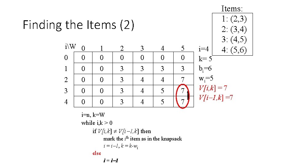
Finding the Items (2) iW 0 0 0 1 0 2 0 3 0 4 0 1 0 0 0 2 0 3 3 3 0 3 4 4 0 3 4 5 5 5 0 3 7 7 7 i=n, k=W while i, k > 0 if V[i, k] V[i 1, k] then mark the ith item as in the knapsack i = i 1, k = k-wi else i = i 1 Items: 1: (2, 3) 2: (3, 4) 3: (4, 5) 4: (5, 6) i=4 k= 5 bi=6 wi=5 V[i, k] = 7 V[i 1, k] =7

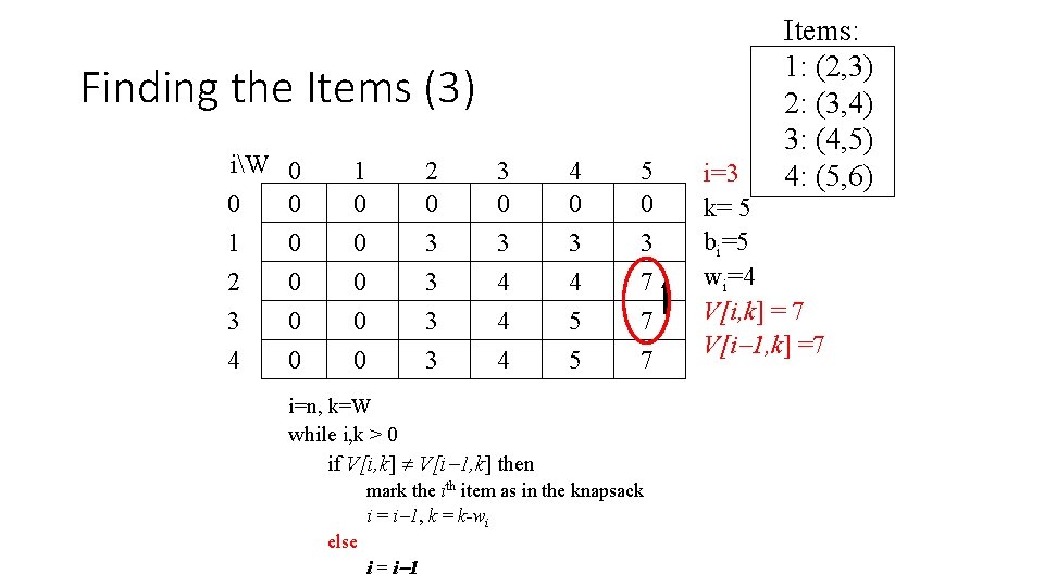
Finding the Items (3) iW 0 0 0 1 0 2 0 3 0 4 0 1 0 0 0 2 0 3 3 3 0 3 4 4 0 3 4 5 5 5 0 3 7 7 7 i=n, k=W while i, k > 0 if V[i, k] V[i 1, k] then mark the ith item as in the knapsack i = i 1, k = k-wi else i = i 1 Items: 1: (2, 3) 2: (3, 4) 3: (4, 5) 4: (5, 6) i=3 k= 5 bi=5 wi=4 V[i, k] = 7 V[i 1, k] =7

Finding the Items (4) iW 0 0 0 1 0 2 0 3 0 4 0 1 0 0 0 2 0 3 3 3 0 3 4 4 0 3 4 5 5 5 0 3 7 7 7 i=n, k=W while i, k > 0 if V[i, k] V[i 1, k] then mark the ith item as in the knapsack i = i 1, k = k-wi else i = i 1 Items: 1: (2, 3) 2: (3, 4) 3: (4, 5) 4: (5, 6) i=2 k= 5 bi=4 wi=3 V[i, k] = 7 V[i 1, k] =3 k wi=2

Finding the Items (5) iW 0 0 0 1 0 2 0 3 0 4 0 1 0 0 0 2 0 3 3 3 0 3 4 4 0 3 4 5 5 5 0 3 7 7 7 i=n, k=W while i, k > 0 if V[i, k] V[i 1, k] then mark the ith item as in the knapsack i = i 1, k = k-wi else i = i 1 Items: 1: (2, 3) 2: (3, 4) 3: (4, 5) 4: (5, 6) i=1 k= 2 bi=3 wi=2 V[i, k] = 3 V[i 1, k] =0 k wi=0

Finding the Items (6) iW 0 0 0 1 0 2 0 3 0 4 0 1 0 0 0 2 0 3 3 3 0 3 4 4 0 3 4 5 5 5 0 3 7 7 7 i=n, k=W while i, k > 0 if V[i, k] V[i 1, k] then mark the nth item as in the knapsack i = i 1, k = k-wi else i = i 1 i=0 k= 0 Items: 1: (2, 3) 2: (3, 4) 3: (4, 5) 4: (5, 6) The optimal knapsack should contain {1, 2}

Finding the Items (7) iW 0 0 0 1 0 2 0 3 0 4 0 1 0 0 0 2 0 3 3 3 0 3 4 4 0 3 4 5 5 5 0 3 7 7 7 i=n, k=W while i, k > 0 if V[i, k] V[i 1, k] then mark the nth item as in the knapsack i = i 1, k = k-wi else i = i 1 Items: 1: (2, 3) 2: (3, 4) 3: (4, 5) 4: (5, 6) The optimal knapsack should contain {1, 2}

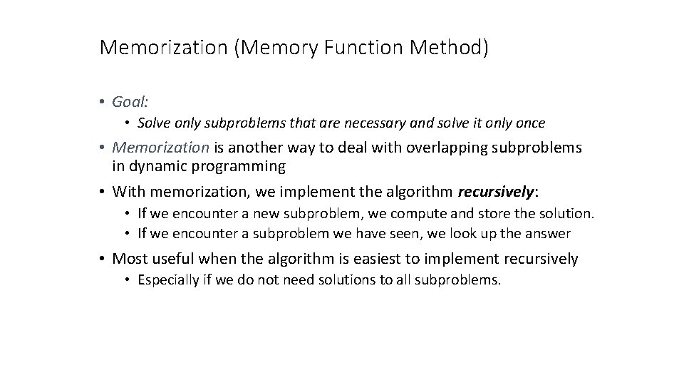
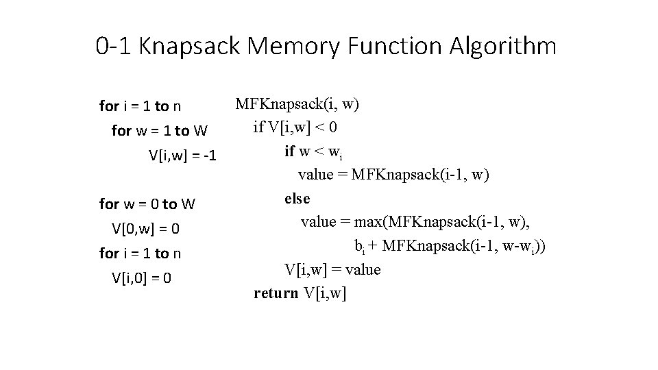
Memorization (Memory Function Method) • Goal: • Solve only subproblems that are necessary and solve it only once • Memorization is another way to deal with overlapping subproblems in dynamic programming • With memorization, we implement the algorithm recursively: • If we encounter a new subproblem, we compute and store the solution. • If we encounter a subproblem we have seen, we look up the answer • Most useful when the algorithm is easiest to implement recursively • Especially if we do not need solutions to all subproblems.

0 -1 Knapsack Memory Function Algorithm for i = 1 to n for w = 1 to W V[i, w] = -1 for w = 0 to W V[0, w] = 0 for i = 1 to n V[i, 0] = 0 MFKnapsack(i, w) if V[i, w] < 0 if w < wi value = MFKnapsack(i-1, w) else value = max(MFKnapsack(i-1, w), bi + MFKnapsack(i-1, w-wi)) V[i, w] = value return V[i, w]

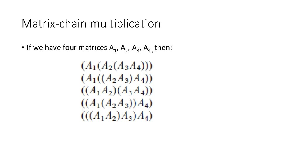
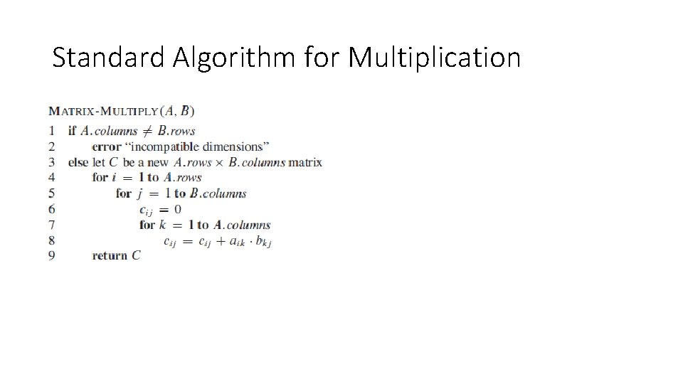
Matrix-chain multiplication • We are given a sequence (chain) (A 1, A 2, …, An) of n matrices to be multiplied, and we wish to compute the product A 1*A 2*…. *An • We can solve this by using the standard algorithm for multiplying pairs of matrices as a subroutine once we have parenthesized it to resolve all ambiguities in how the matrices are multiplied together. • A product of matrices is fully parenthesized if it is either a single matrix or the product of two fully parenthesized matrix products, surrounded by parentheses.

Matrix-chain multiplication • If we have four matrices A 1, A 2, A 3, A 4 , then:

Standard Algorithm for Multiplication

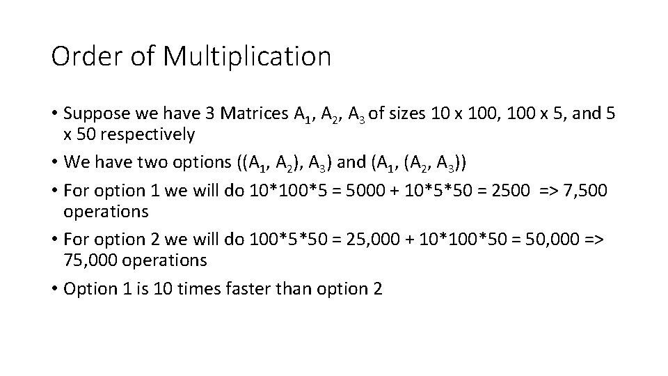
Order of Multiplication • Suppose we have 3 Matrices A 1, A 2, A 3 of sizes 10 x 100, 100 x 5, and 5 x 50 respectively • We have two options ((A 1, A 2), A 3) and (A 1, (A 2, A 3)) • For option 1 we will do 10*100*5 = 5000 + 10*5*50 = 2500 => 7, 500 operations • For option 2 we will do 100*5*50 = 25, 000 + 10*100*50 = 50, 000 => 75, 000 operations • Option 1 is 10 times faster than option 2

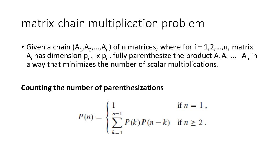
matrix-chain multiplication problem • Given a chain (A 1, A 2, …, An) of n matrices, where for i = 1, 2, …, n, matrix Ai has dimension pi-1 x pi , fully parenthesize the product A 1 A 2 … An in a way that minimizes the number of scalar multiplications. Counting the number of parenthesizations

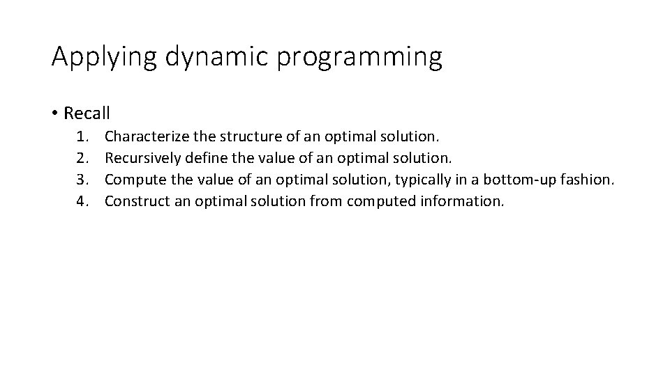
Applying dynamic programming • Recall 1. 2. 3. 4. Characterize the structure of an optimal solution. Recursively define the value of an optimal solution. Compute the value of an optimal solution, typically in a bottom-up fashion. Construct an optimal solution from computed information.

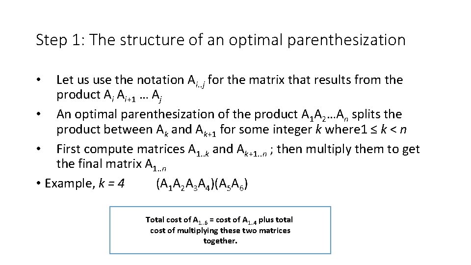
Step 1: The structure of an optimal parenthesization Let us use the notation Ai. . j for the matrix that results from the product Ai Ai+1 … Aj • An optimal parenthesization of the product A 1 A 2…An splits the product between Ak and Ak+1 for some integer k where 1 ≤ k < n • First compute matrices A 1. . k and Ak+1. . n ; then multiply them to get the final matrix A 1. . n • Example, k = 4 (A 1 A 2 A 3 A 4)(A 5 A 6) • Total cost of A 1. . 6 = cost of A 1. . 4 plus total cost of multiplying these two matrices together.

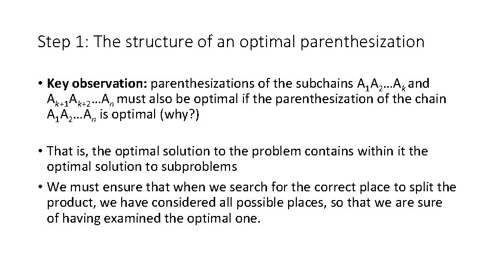
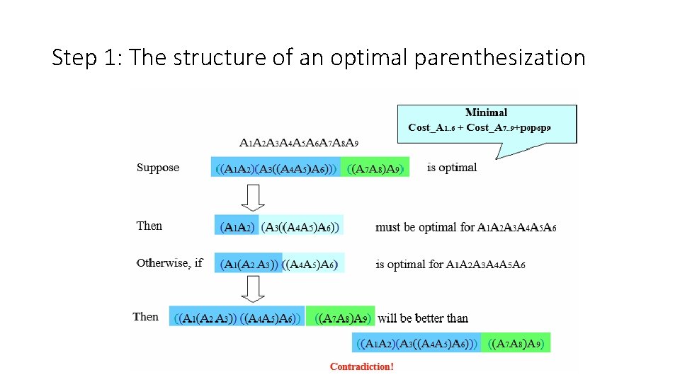
Step 1: The structure of an optimal parenthesization • Key observation: parenthesizations of the subchains A 1 A 2…Ak and Ak+1 Ak+2…An must also be optimal if the parenthesization of the chain A 1 A 2…An is optimal (why? ) • That is, the optimal solution to the problem contains within it the optimal solution to subproblems • We must ensure that when we search for the correct place to split the product, we have considered all possible places, so that we are sure of having examined the optimal one.

Step 1: The structure of an optimal parenthesization

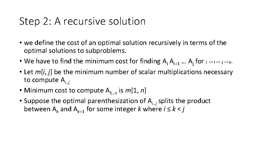
Step 2: A recursive solution • we define the cost of an optimal solution recursively in terms of the optimal solutions to subproblems. • We have to find the minimum cost for finding Ai Ai+1 … Aj for 1 <= i <= j <= n. • Let m[i, j] be the minimum number of scalar multiplications necessary to compute Ai. . j • Minimum cost to compute A 1. . n is m[1, n] • Suppose the optimal parenthesization of Ai. . j splits the product between Ak and Ak+1 for some integer k where i ≤ k < j

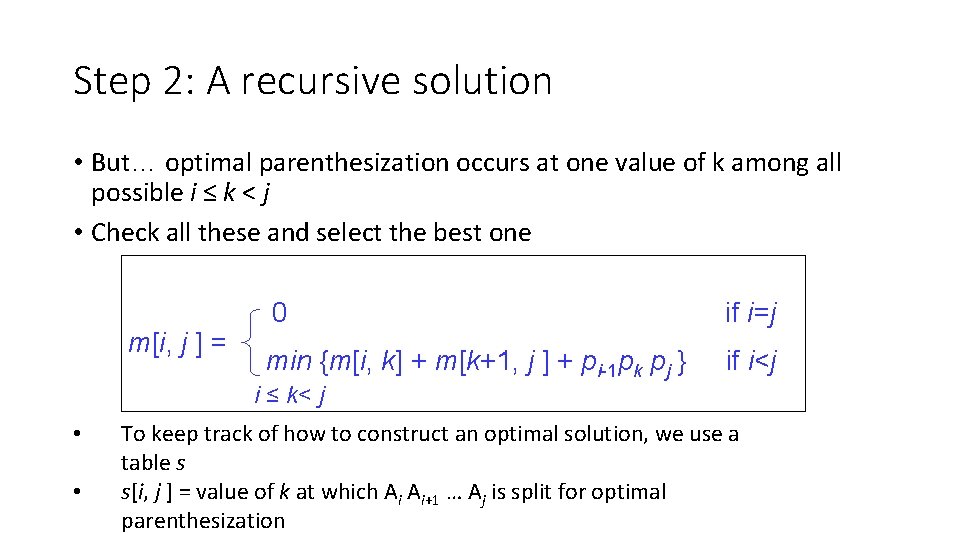
Step 2: A recursive solution • We can define m[i, j] recursively as follows. If i = j , the problem is trivial; • To compute m[i, j] for i < j, we observe • Ai. . j = (Ai Ai+1…Ak)·(Ak+1 Ak+2…Aj)= Ai. . k · Ak+1. . j • Cost of computing Ai. . j = cost of computing Ai. . k + cost of computing Ak+1. . j + cost of multiplying Ai. . k and Ak+1. . j • Cost of multiplying Ai. . k and Ak+1. . j is pi-1 pk pj m[i, j ] = m[i, k] + m[k+1, j ] + pi-1 pk pj for i ≤ k < j • m[i, i ] = 0 for i=1, 2, …, n

Step 2: A recursive solution • But… optimal parenthesization occurs at one value of k among all possible i ≤ k < j • Check all these and select the best one m[i, j ] = 0 if i=j min {m[i, k] + m[k+1, j ] + pi-1 pk pj } if i<j i ≤ k< j • • To keep track of how to construct an optimal solution, we use a table s s[i, j ] = value of k at which Ai Ai+1 … Aj is split for optimal parenthesization

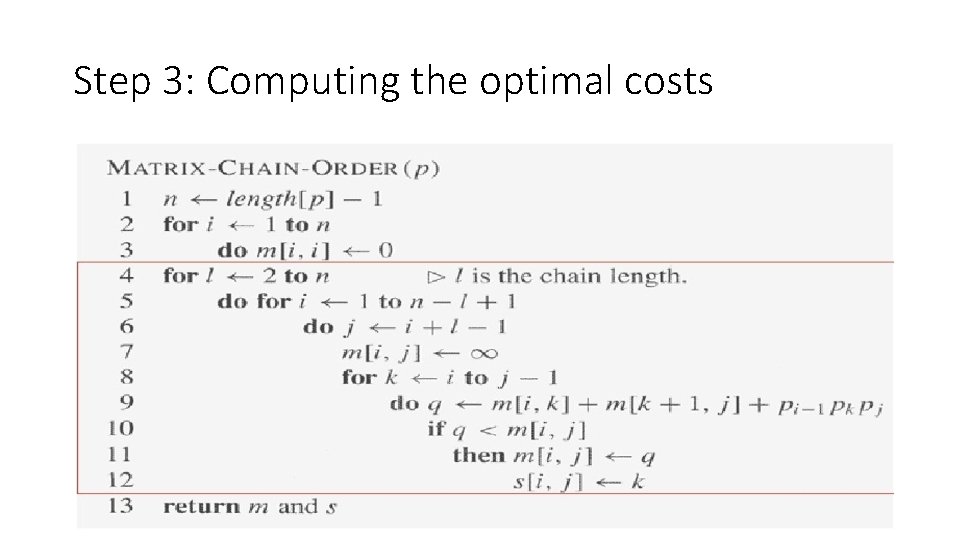
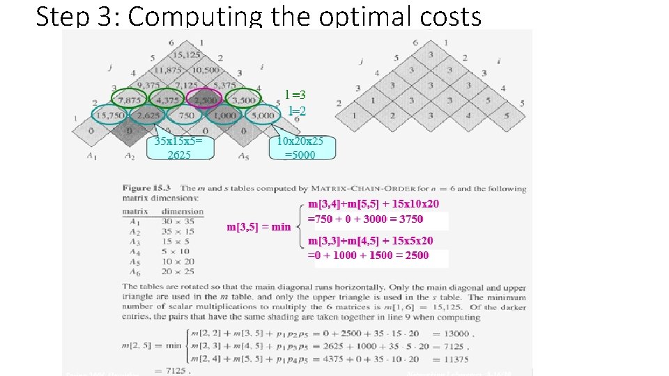
Step 3: Computing the optimal costs Input: Array p[0…n] containing matrix dimensions and n Result: Minimum-cost table m and split table s MATRIX-CHAIN-ORDER(p[ ], n) for i ← 1 to n Takes O(n 3) time m[i, i] ← 0 for l ← 2 to n Requires O(n 2) space for i ← 1 to n-l+1 j ← i+l-1 m[i, j] ← for k ← i to j-1 q ← m[i, k] + m[k+1, j] + p[i-1] p[k] p[j] if q < m[i, j] ← q s[i, j] ← k return m and s

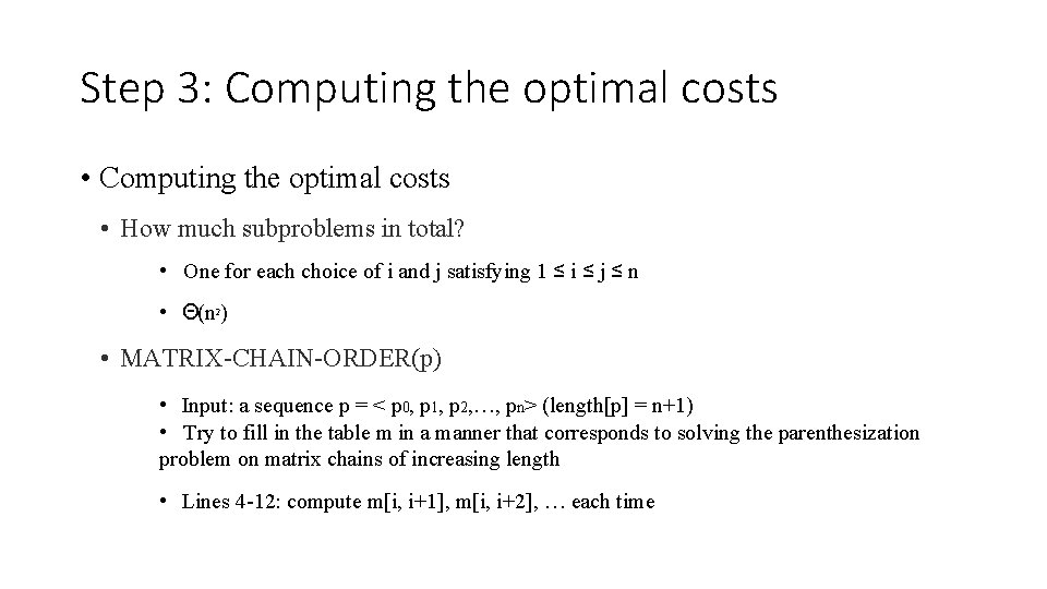
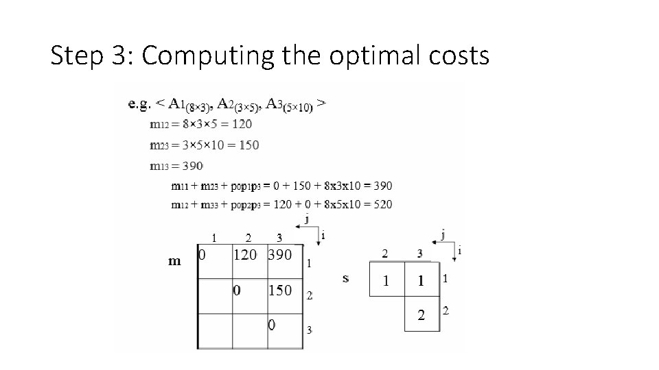
Step 3: Computing the optimal costs • How much subproblems in total? • One for each choice of i and j satisfying 1 ≤ i ≤ j ≤ n • Θ(n 2) • MATRIX-CHAIN-ORDER(p) • Input: a sequence p = < p 0, p 1, p 2, …, pn> (length[p] = n+1) • Try to fill in the table m in a manner that corresponds to solving the parenthesization problem on matrix chains of increasing length • Lines 4 -12: compute m[i, i+1], m[i, i+2], … each time

Step 3: Computing the optimal costs

Step 3: Computing the optimal costs

Step 3: Computing the optimal costs

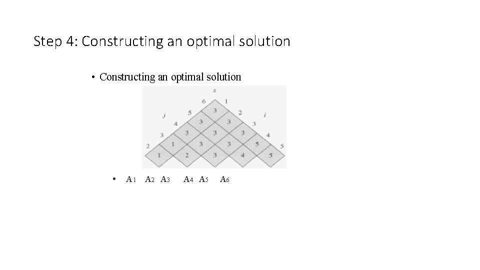
Step 4: Constructing an optimal solution • Each entry s[i, j] records the value of k such that the optimal parenthesization of Ai. Ai+1…Aj splits the product between Ak and Ak+1 • • • A 1. . n →A 1. . s[1. . n] As[1. . n]+1. . n A 1. . s[1. . n] →A 1. . s[1, s[1. . n]] As[1, s[1. . n]]+1. . s[1. . n] Recursive…

Step 4: Constructing an optimal solution • Constructing an optimal solution • A 1 A 2 A 3 A 4 A 5 A 6

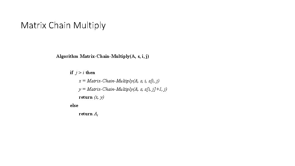
Matrix Chain Multiply Algorithm Matrix-Chain-Multiply(A, s, i, j) if j > i then x = Matrix-Chain-Multiply(A, s, i, s[i, j) y = Matrix-Chain-Multiply(A, s, s[i, j]+1, j) return (x, y) else return Ai

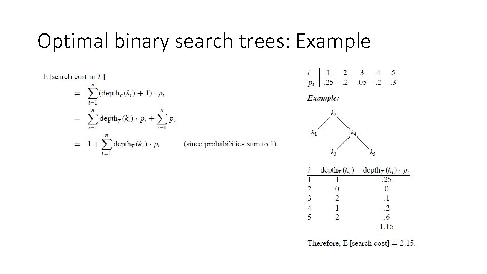
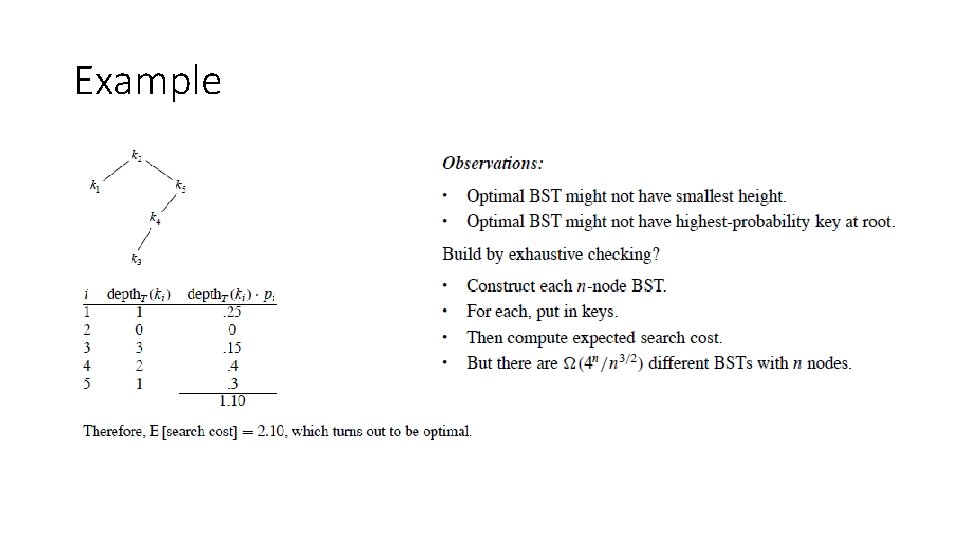
Optimal binary search trees • Given sequence K = k 1, k 2, . . . , kn of n distinct keys, sorted (k 1 < k 2 < · · · < kn). • Want to build a binary search tree from the keys. • For ki , have probability pi that a search is for ki. • Want BST with minimum expected search cost.

Optimal binary search trees: Example

Example

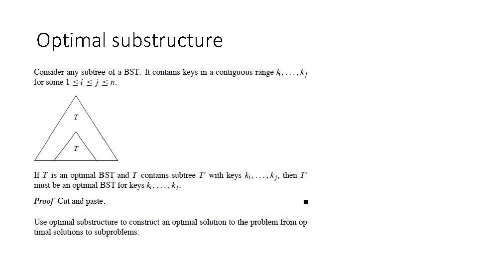
Optimal substructure

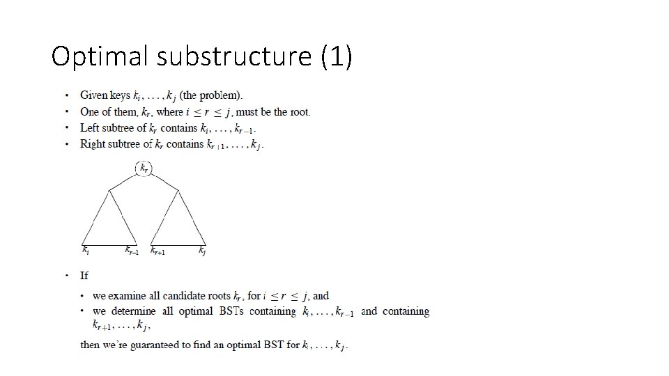
Optimal substructure (1)

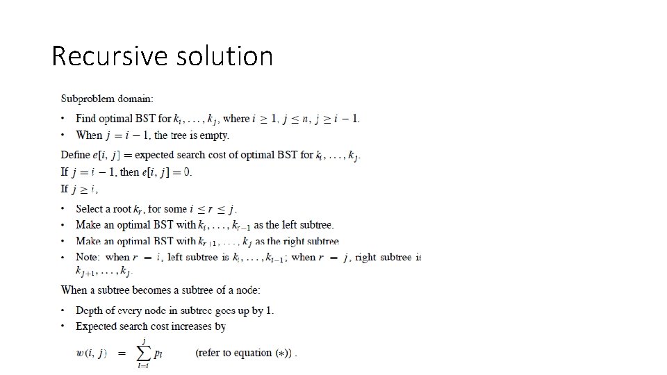
Recursive solution

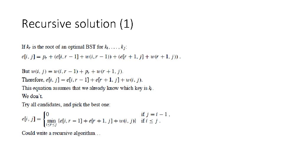
Recursive solution (1)

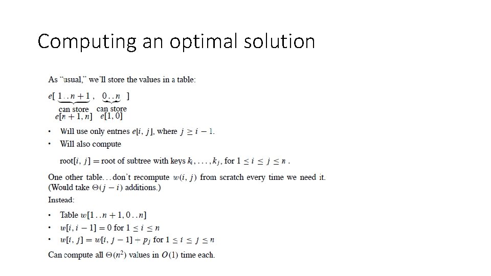
Computing an optimal solution

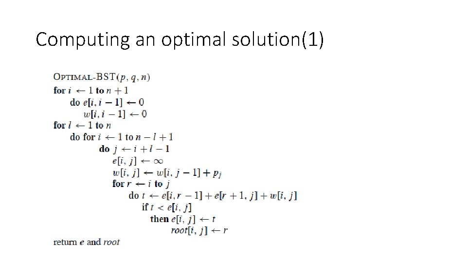
Computing an optimal solution(1)

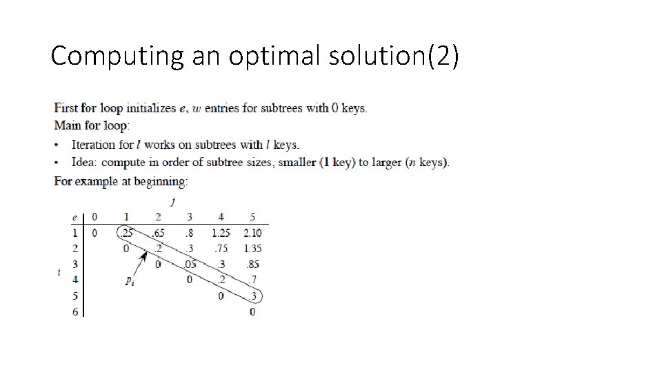
Computing an optimal solution(2)

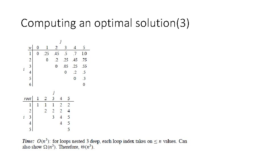
Computing an optimal solution(3)

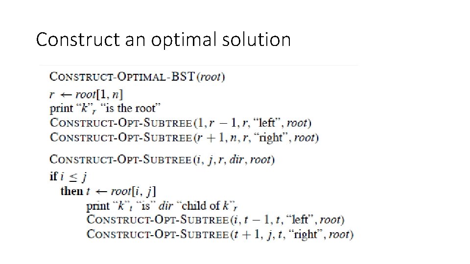
Construct an optimal solution

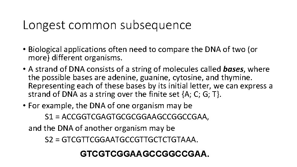
Longest common subsequence • Biological applications often need to compare the DNA of two (or more) different organisms. • A strand of DNA consists of a string of molecules called bases, where the possible bases are adenine, guanine, cytosine, and thymine. Representing each of these bases by its initial letter, we can express a strand of DNA as a string over the finite set {A; C; G; T}. • For example, the DNA of one organism may be S 1 = ACCGGTCGAGTGCGCGGAAGCCGAA, and the DNA of another organism may be S 2 = GTCGTTCGGAATGCCGTTGCTCTGTAAA. GTCGTCGGAAGCCGAA.

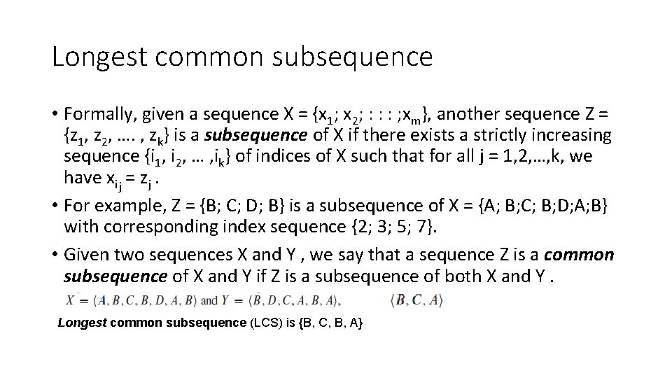
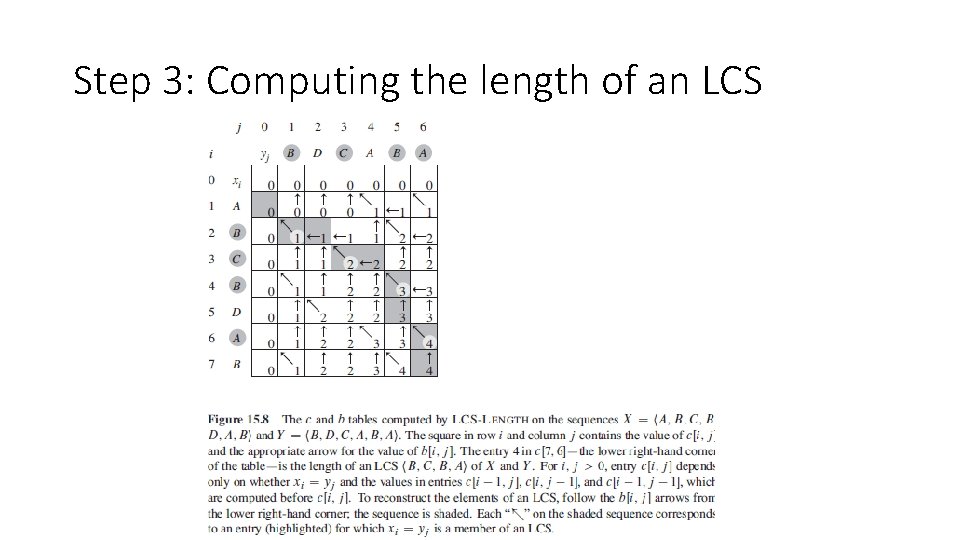
Longest common subsequence • Formally, given a sequence X = {x 1; x 2; : : : ; xm}, another sequence Z = {z 1, z 2, …. , zk} is a subsequence of X if there exists a strictly increasing sequence {i 1, i 2, … , ik} of indices of X such that for all j = 1, 2, …, k, we have xij = zj. • For example, Z = {B; C; D; B} is a subsequence of X = {A; B; C; B; D; A; B} with corresponding index sequence {2; 3; 5; 7}. • Given two sequences X and Y , we say that a sequence Z is a common subsequence of X and Y if Z is a subsequence of both X and Y. Longest common subsequence (LCS) is {B, C, B, A}

longest-common-subsequence problem • we are given two sequences X = {x 1; x 2; : : : ; xm} and Y = {y 1; y 2; : : : ; yn} and wish to find a maximum length common subsequence of X and Y.

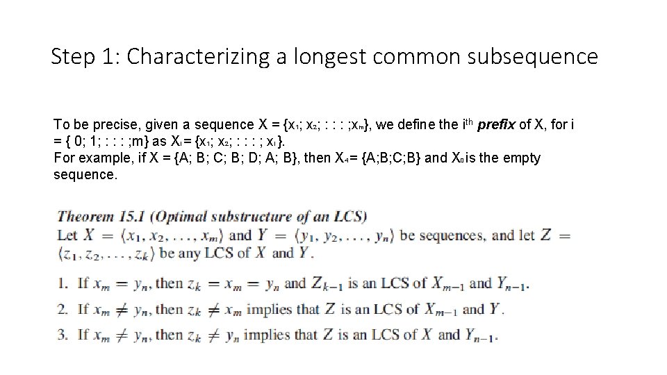
Step 1: Characterizing a longest common subsequence To be precise, given a sequence X = {x 1; x 2; : : : ; xm}, we define the ith prefix of X, for i = { 0; 1; : : : ; m} as Xi = {x 1; x 2; : : : ; xi }. For example, if X = {A; B; C; B; D; A; B}, then X 4 = {A; B; C; B} and X 0 is the empty sequence.

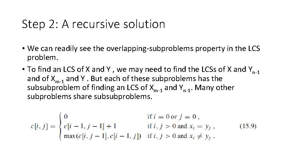
Step 2: A recursive solution • We can readily see the overlapping-subproblems property in the LCS problem. • To find an LCS of X and Y , we may need to find the LCSs of X and Yn-1 and of Xm-1 and Y. But each of these subproblems has the subsubproblem of finding an LCS of Xm-1 and Yn-1. Many other subproblems share subsubproblems.

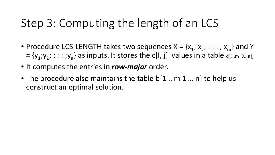
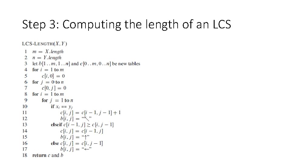
Step 3: Computing the length of an LCS • Procedure LCS-LENGTH takes two sequences X = {x 1; x 2; : : : ; xm} and Y = {y 1; y 2; : : : ; yn} as inputs. It stores the c[I, j] values in a table c[0. . m 0. . n], • It computes the entries in row-major order. • The procedure also maintains the table b[1. . m 1 … n] to help us construct an optimal solution.

Step 3: Computing the length of an LCS

Step 3: Computing the length of an LCS

Step 4: Constructing an LCS