Chapter 4 Properties of the Least Squares Estimator

Chapter 4: Properties of the Least Squares Estimator In this chapter, we will • Review the formulas for b 1 and b 2 • Derive their means, variances and probability density functions • To do so, we will use the assumptions we made in Chapter 3. • Do a Monte Carlo simulation to demonstrate the idea of a sampling distribution. 4. 1

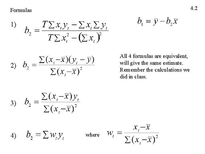
4. 2 Formulas 1) All 4 formulas are equivalent, will give the same estimate. Remember the calculations we did in class. 2) 3) 4) where

Properties of the Least Squares Estimators Introduction From Chapter 3: • The population parameters 1 and 2 are unknown population parameters that must be estimated • The Method of Least Squares gives us formulas for b 1 and b 2, the estimators for 1 and 2 In Chapter 4: • Recognize that these estimators are random variables We want to know their mean, variance and shape First, review the assumptions of the model from Ch. 3 4. 3

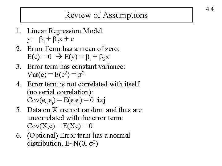
Review of Assumptions 1. Linear Regression Model y = 1 + 2 x + e 2. Error Term has a mean of zero: E(e) = 0 E(y) = 1 + 2 x 3. Error term has constant variance: Var(e) = E(e 2) = 2 4. Error term is not correlated with itself (no serial correlation): Cov(ei, ej) = E(eiej) = 0 i j 5. Data on X are not random and thus are uncorrelated with the error term: Cov(X, e) = E(Xe) = 0 6. (Optional) Error term has a normal distribution. E~N(0, 2) 4. 4

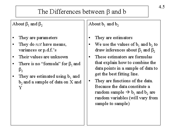
The Differences between and b About 1 and 2 About b 1 and b 2 • They are parameters • They do not have means, variances or p. d. f. ’s • Their values are unknown • There is no “formula” for 1 and 2 • They are estimated using b 1 and b 2 and a sample of data on X and Y • They are estimators • We use the values of b 1 and b 2 to draw inferences about 1 and 2 • These estimators are formulas that explain how to combine the data points in a sample of data to get the best fitting line. • They are functions of the data. Because the data constitute a random sample b 1 and b 2 are random variables (will vary from sample to sample) 4. 5

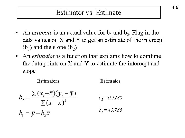
Estimator vs. Estimate • An estimate is an actual value for b 1 and b 2. Plug in the data values on X and Y to get an estimate of the intercept (b 1) and the slope (b 2) • An estimator is a function that explains how to combine the data points on X and Y to estimate the intercept and slope Estimators Estimates b 2= 0. 1283 b 1= 40. 768 4. 6

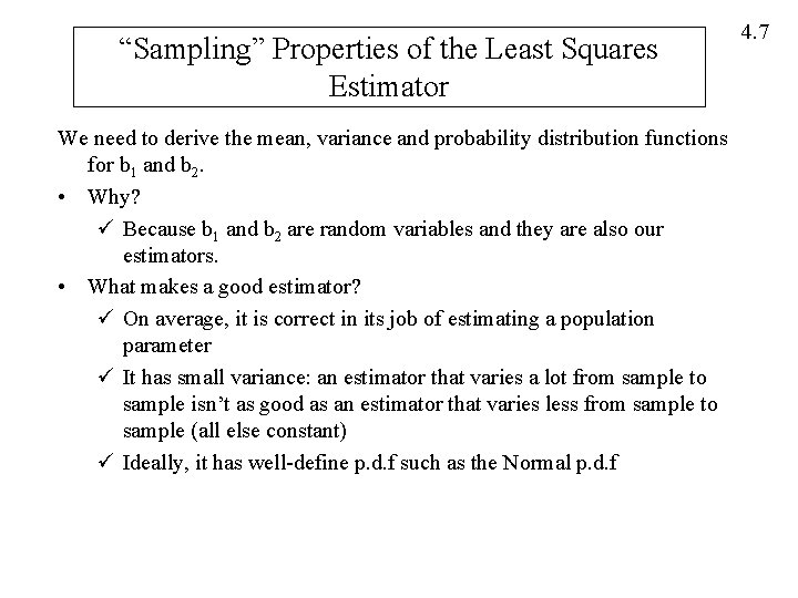
“Sampling” Properties of the Least Squares Estimator We need to derive the mean, variance and probability distribution functions for b 1 and b 2. • Why? ü Because b 1 and b 2 are random variables and they are also our estimators. • What makes a good estimator? ü On average, it is correct in its job of estimating a population parameter ü It has small variance: an estimator that varies a lot from sample to sample isn’t as good as an estimator that varies less from sample to sample (all else constant) ü Ideally, it has well-define p. d. f such as the Normal p. d. f 4. 7

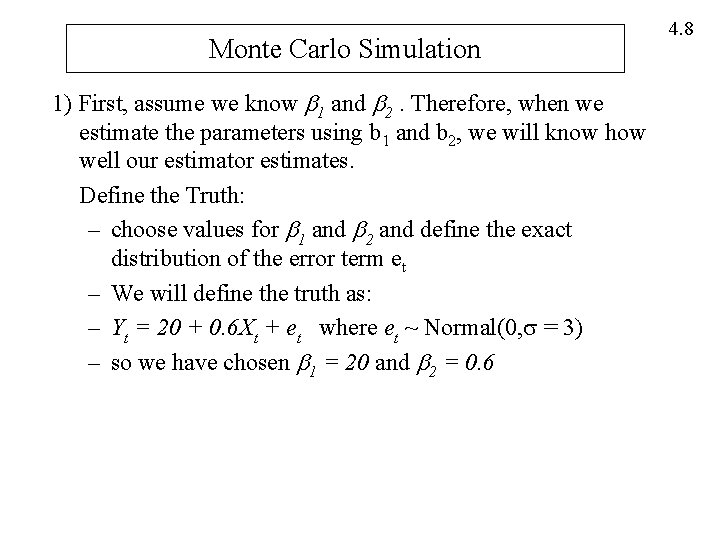
Monte Carlo Simulation 1) First, assume we know 1 and 2. Therefore, when we estimate the parameters using b 1 and b 2, we will know how well our estimator estimates. Define the Truth: – choose values for 1 and 2 and define the exact distribution of the error term et – We will define the truth as: – Yt = 20 + 0. 6 Xt + et where et ~ Normal(0, = 3) – so we have chosen 1 = 20 and 2 = 0. 6 4. 8

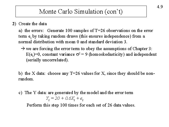
Monte Carlo Simulation (con’t) 2) Create the data a) the errors: Generate 100 samples of T=26 observations on the error term et by taking random draws (this ensures independence) from a normal distribution with mean 0 and standard deviation 3. we are forcing the error term to obey the assumptions of Chapter 3: E(et)=0, constant variance 2 = 9 (homoskedasticity) and independent (serially uncorrelated). b) the X data: choose any T=26 values for X, since they should be nonrandom. c) The Y data: are generated by the model and the error term Yt = 20 + 0. 6 Xt + et Perform this step 100 times for each set of 26 data values. 4. 9

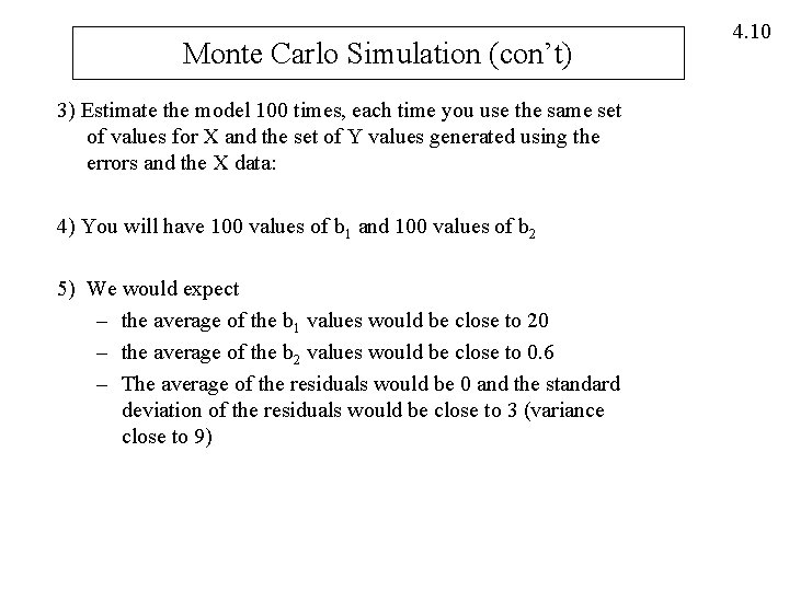
Monte Carlo Simulation (con’t) 3) Estimate the model 100 times, each time you use the same set of values for X and the set of Y values generated using the errors and the X data: 4) You will have 100 values of b 1 and 100 values of b 2 5) We would expect – the average of the b 1 values would be close to 20 – the average of the b 2 values would be close to 0. 6 – The average of the residuals would be 0 and the standard deviation of the residuals would be close to 3 (variance close to 9) 4. 10

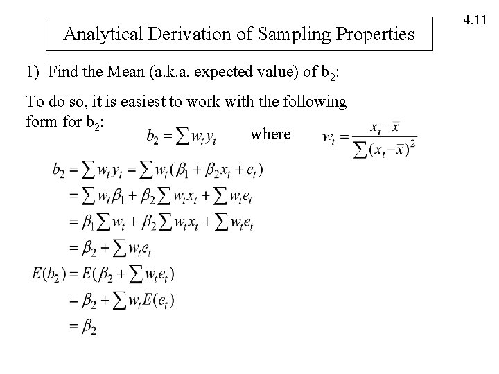
Analytical Derivation of Sampling Properties 1) Find the Mean (a. k. a. expected value) of b 2: To do so, it is easiest to work with the following form for b 2: where 4. 11

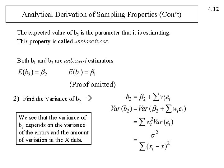
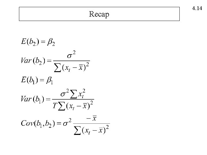
Analytical Derivation of Sampling Properties (Con’t) The expected value of b 2 is the parameter that it is estimating. This property is called unbiasedness. Both b 1 and b 2 are unbiased estimators (Proof omitted) 2) Find the Variance of b 2 We see that the variance of b 2 depends on the variance of the errors and the amount of variation in the X data. 4. 12

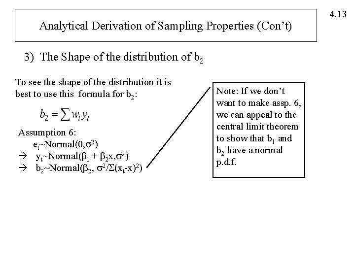
Analytical Derivation of Sampling Properties (Con’t) 3) The Shape of the distribution of b 2 To see the shape of the distribution it is best to use this formula for b 2: Assumption 6: et~Normal(0, 2) yt~Normal( 1 + 2 x, 2) b 2~Normal( 2, 2/ (xt-x)2) Note: If we don’t want to make assp. 6, we can appeal to the central limit theorem to show that b 1 and b 2 have a normal p. d. f. 4. 13

Recap 4. 14

4. 15 About the variance formulas: We want our estimators to be precise. High precision means low variance. The variances of b 1 and b 2 are affected by: • The variance of the error term. If the error term has small variance, our estimator will be more precise. • The amount of variation in the X data. If there is lots of variation in the X data, our estimator will be more precise. (see graph, p. 75) • The size of the sample (T). The larger the sample, the more precise the estimator.

Gauss Markov Theorem This is a theorem that tells us that the least squares estimator is the best one available: “Under the assumptions 1 -5 (the 6 th assumption isn’t needed for theorem to be true) of the linear regression model, the least squares estimators b 1 and b 2 have the smallest variance of all linear and unbiased estimators of 1 and 2. They are the BLUE (Best, linear, unbiased, estimator). ” 4. 16

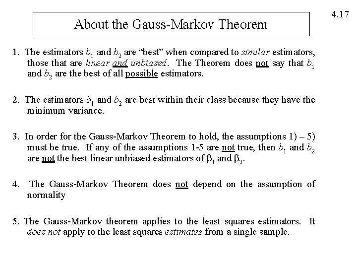
About the Gauss-Markov Theorem 1. The estimators b 1 and b 2 are “best” when compared to similar estimators, those that are linear and unbiased. Theorem does not say that b 1 and b 2 are the best of all possible estimators. 2. The estimators b 1 and b 2 are best within their class because they have the minimum variance. 3. In order for the Gauss-Markov Theorem to hold, the assumptions 1) – 5) must be true. If any of the assumptions 1 -5 are not true, then b 1 and b 2 are not the best linear unbiased estimators of 1 and 2. 4. The Gauss-Markov Theorem does not depend on the assumption of normality 5. The Gauss-Markov theorem applies to the least squares estimators. It does not apply to the least squares estimates from a single sample. 4. 17

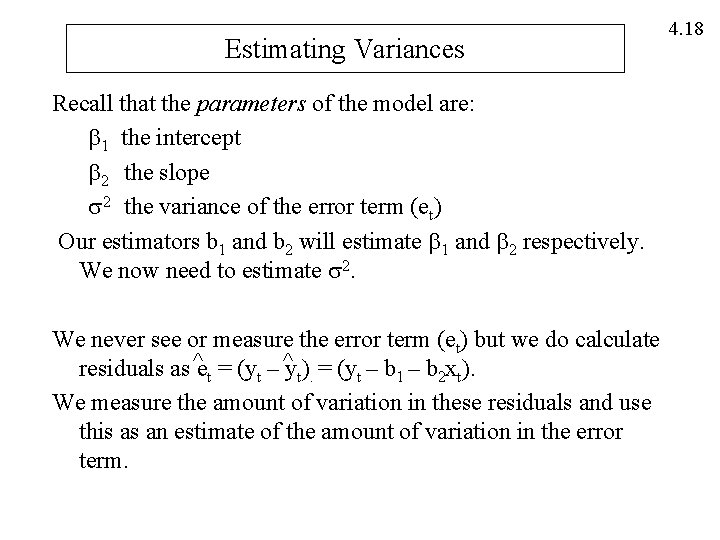
Estimating Variances Recall that the parameters of the model are: 1 the intercept 2 the slope 2 the variance of the error term (et) Our estimators b 1 and b 2 will estimate 1 and 2 respectively. We now need to estimate 2. We never see or measure the error term (et) but we do calculate residuals as ^et = (yt – ^yt). = (yt – b 1 – b 2 xt). We measure the amount of variation in these residuals and use this as an estimate of the amount of variation in the error term. 4. 18

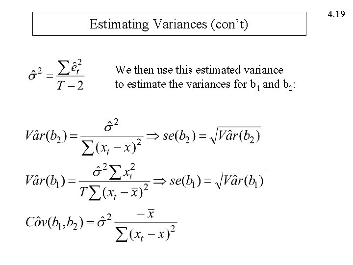
Estimating Variances (con’t) We then use this estimated variance to estimate the variances for b 1 and b 2: 4. 19