Markov Random Fields and Segmentation with Graph Cuts

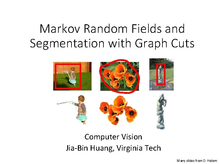
Markov Random Fields and Segmentation with Graph Cuts Computer Vision Jia-Bin Huang, Virginia Tech Many slides from D. Hoiem

Administrative stuffs • Final project • Proposal due Oct 27 (Thursday) • HW 4 is out • Due 11: 59 pm on Wed, November 2 nd, 2016

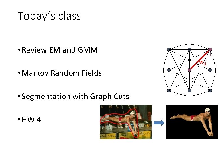
Today’s class • Review EM and GMM wij • Markov Random Fields • Segmentation with Graph Cuts • HW 4 j i

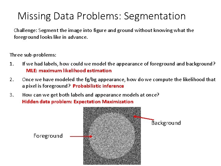
Missing Data Problems: Segmentation Challenge: Segment the image into figure and ground without knowing what the foreground looks like in advance. Three sub-problems: 1. If we had labels, how could we model the appearance of foreground and background? MLE: maximum likelihood estimation 2. Once we have modeled the fg/bg appearance, how do we compute the likelihood that a pixel is foreground? Probabilistic inference 3. How can we get both labels and appearance models at once? Hidden data problem: Expectation Maximization Background Foreground

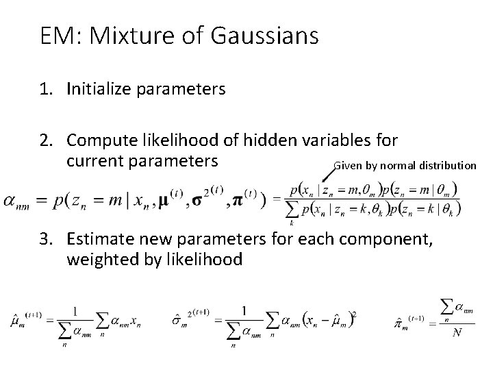
EM: Mixture of Gaussians 1. Initialize parameters 2. Compute likelihood of hidden variables for current parameters Given by normal distribution 3. Estimate new parameters for each component, weighted by likelihood

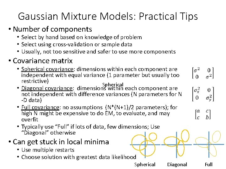
Gaussian Mixture Models: Practical Tips • Number of components • Select by hand based on knowledge of problem • Select using cross-validation or sample data • Usually, not too sensitive and safer to use more components • Covariance matrix • Spherical covariance: dimensions within each component are independent with equal variance (1 parameter but usually too restrictive) Spherical • Diagonal covariance: dimensions within each component are not independent with difference variances (N parameters for N -D data) • Full covariance: no assumptions (N*(N+1)/2 parameters); for high N might be expensive to do EM, to evaluate, and may overfit • Typically use “Full” if lots of data, few dimensions; Use “Diagonal” otherwise • Can get stuck in local minima • Use multiple restarts • Choose solution with greatest data likelihood Spherical Diagonal Full

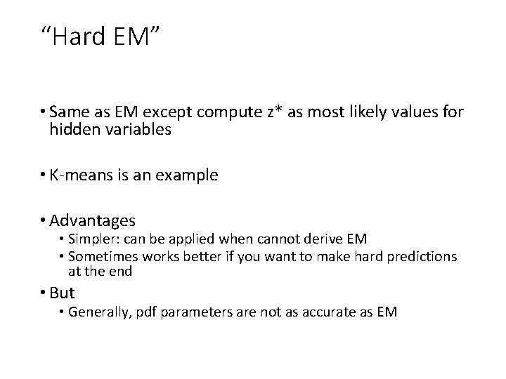
“Hard EM” • Same as EM except compute z* as most likely values for hidden variables • K-means is an example • Advantages • Simpler: can be applied when cannot derive EM • Sometimes works better if you want to make hard predictions at the end • But • Generally, pdf parameters are not as accurate as EM

EM Demo • GMM with images demos

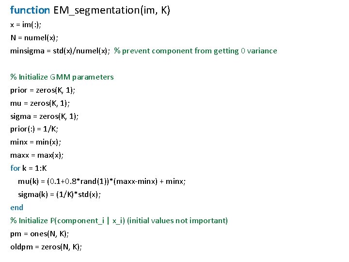
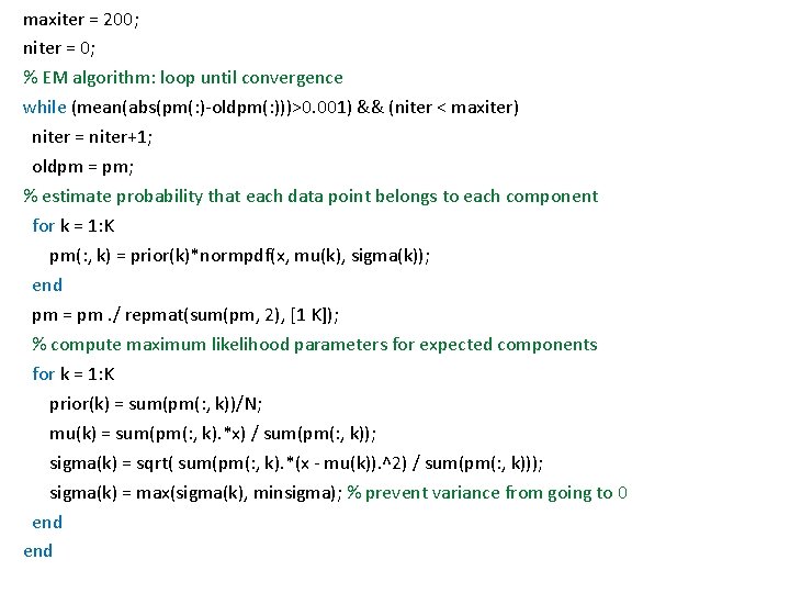
function EM_segmentation(im, K) x = im(: ); N = numel(x); minsigma = std(x)/numel(x); % prevent component from getting 0 variance % Initialize GMM parameters prior = zeros(K, 1); mu = zeros(K, 1); sigma = zeros(K, 1); prior(: ) = 1/K; minx = min(x); maxx = max(x); for k = 1: K mu(k) = (0. 1+0. 8*rand(1))*(maxx-minx) + minx; sigma(k) = (1/K)*std(x); end % Initialize P(component_i | x_i) (initial values not important) pm = ones(N, K); oldpm = zeros(N, K);

maxiter = 200; niter = 0; % EM algorithm: loop until convergence while (mean(abs(pm(: )-oldpm(: )))>0. 001) && (niter < maxiter) niter = niter+1; oldpm = pm; % estimate probability that each data point belongs to each component for k = 1: K pm(: , k) = prior(k)*normpdf(x, mu(k), sigma(k)); end pm = pm. / repmat(sum(pm, 2), [1 K]); % compute maximum likelihood parameters for expected components for k = 1: K prior(k) = sum(pm(: , k))/N; mu(k) = sum(pm(: , k). *x) / sum(pm(: , k)); sigma(k) = sqrt( sum(pm(: , k). *(x - mu(k)). ^2) / sum(pm(: , k))); sigma(k) = max(sigma(k), minsigma); % prevent variance from going to 0 end

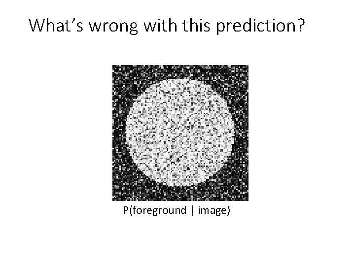
What’s wrong with this prediction? P(foreground | image)

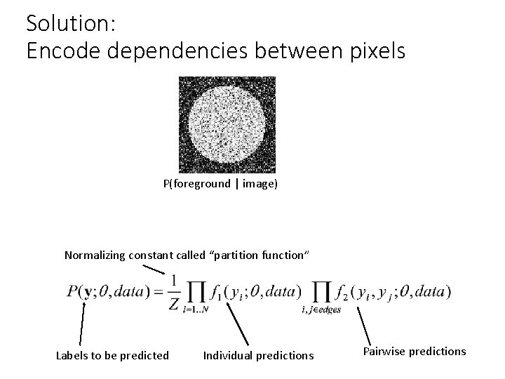
Solution: Encode dependencies between pixels P(foreground | image) Normalizing constant called “partition function” Labels to be predicted Individual predictions Pairwise predictions

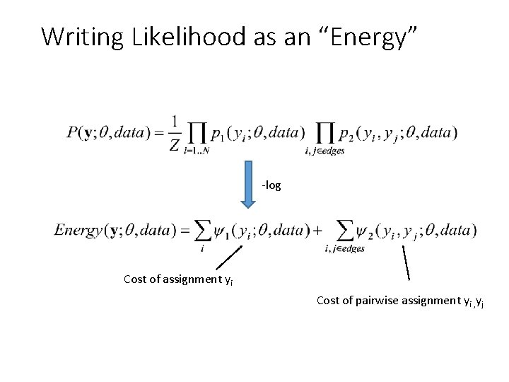
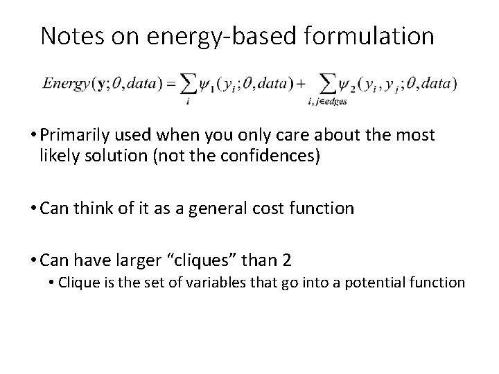
Writing Likelihood as an “Energy” -log Cost of assignment yi Cost of pairwise assignment yi , yj

Notes on energy-based formulation • Primarily used when you only care about the most likely solution (not the confidences) • Can think of it as a general cost function • Can have larger “cliques” than 2 • Clique is the set of variables that go into a potential function

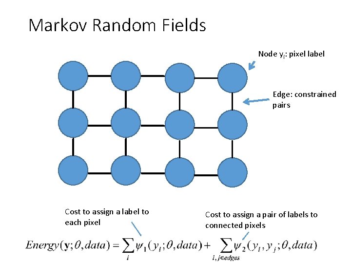
Markov Random Fields Node yi: pixel label Edge: constrained pairs Cost to assign a label to each pixel Cost to assign a pair of labels to connected pixels

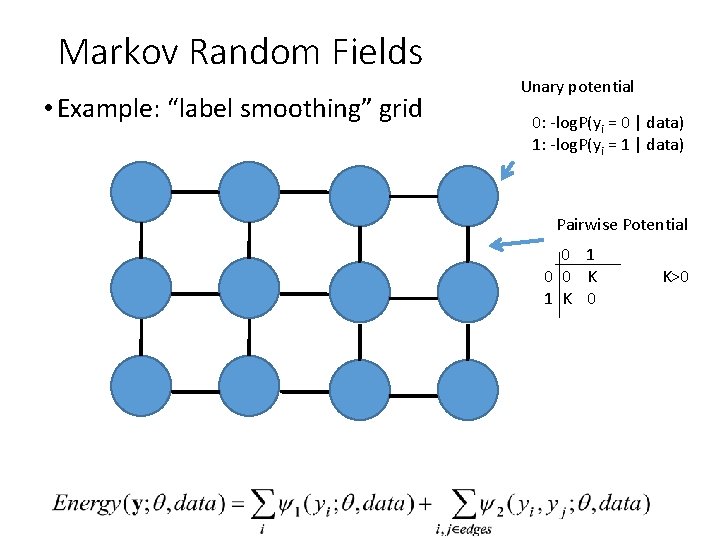
Markov Random Fields • Example: “label smoothing” grid Unary potential 0: -log. P(yi = 0 | data) 1: -log. P(yi = 1 | data) Pairwise Potential 0 1 0 0 K 1 K 0 K>0

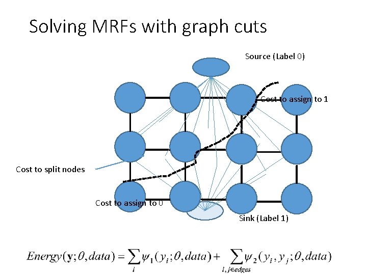
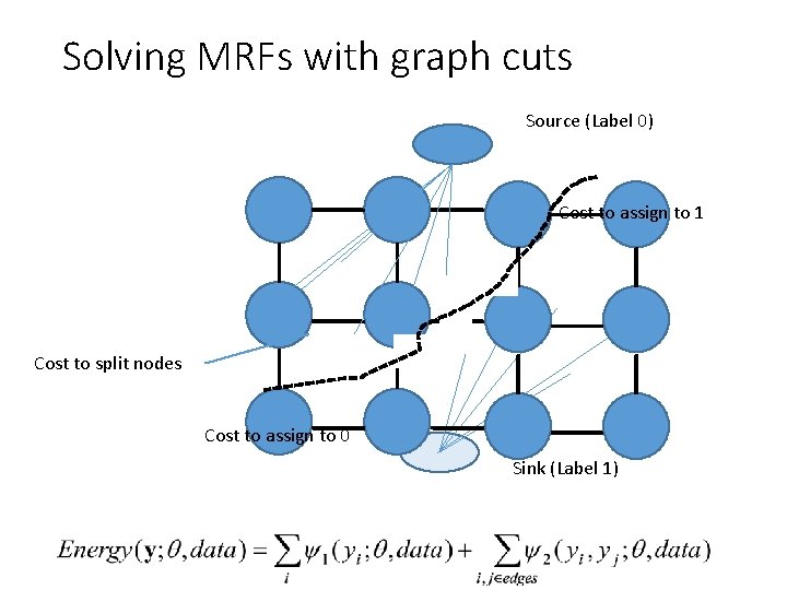
Solving MRFs with graph cuts Source (Label 0) Cost to assign to 1 Cost to split nodes Cost to assign to 0 Sink (Label 1)

Solving MRFs with graph cuts Source (Label 0) Cost to assign to 1 Cost to split nodes Cost to assign to 0 Sink (Label 1)

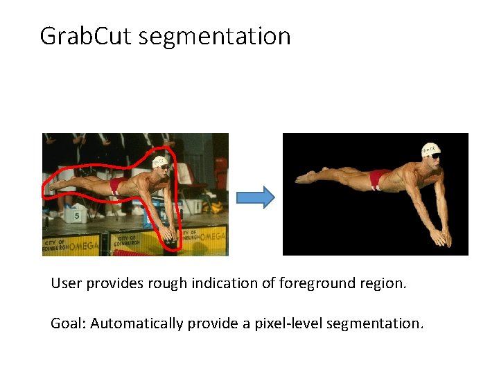
Grab. Cut segmentation User provides rough indication of foreground region. Goal: Automatically provide a pixel-level segmentation.

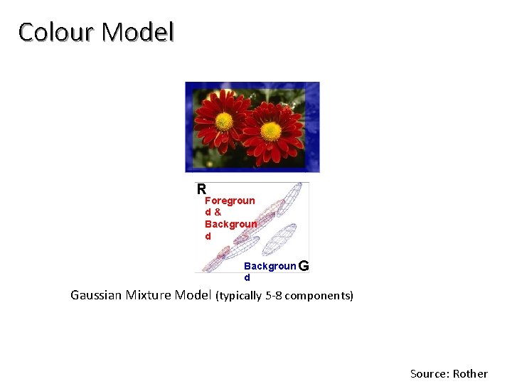
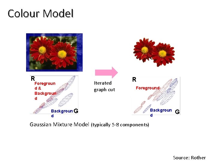
Colour Model R Foregroun d& Backgroun d Backgroun G d Gaussian Mixture Model (typically 5 -8 components) Source: Rother

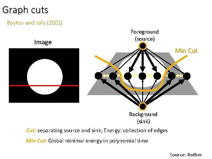
Graph cuts Boykov and Jolly (2001) Image Foreground (source) Min Cut Background (sink) Cut: separating source and sink; Energy: collection of edges Min Cut: Global minimal energy in polynomial time Source: Rother

Colour Model R Foregroun d& Backgroun d Iterated graph cut R Foreground Backgroun G d Backgroun d G Gaussian Mixture Model (typically 5 -8 components) Source: Rother

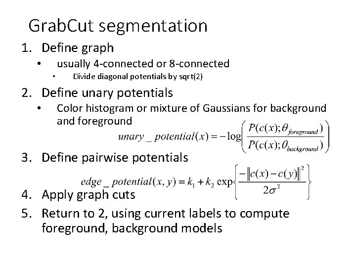
Grab. Cut segmentation 1. Define graph usually 4 -connected or 8 -connected • • Divide diagonal potentials by sqrt(2) 2. Define unary potentials • Color histogram or mixture of Gaussians for background and foreground 3. Define pairwise potentials 4. Apply graph cuts 5. Return to 2, using current labels to compute foreground, background models

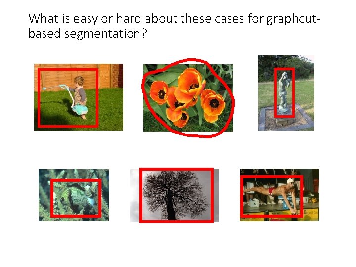
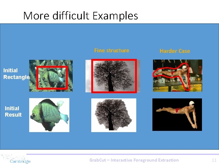
What is easy or hard about these cases for graphcutbased segmentation?

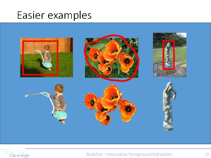
Easier examples Grab. Cut – Interactive Foreground Extraction 10

More difficult Examples Fine structure Harder Case Camouflage & Initial Rectangle Low Contrast Initial Result Grab. Cut – Interactive Foreground Extraction 11

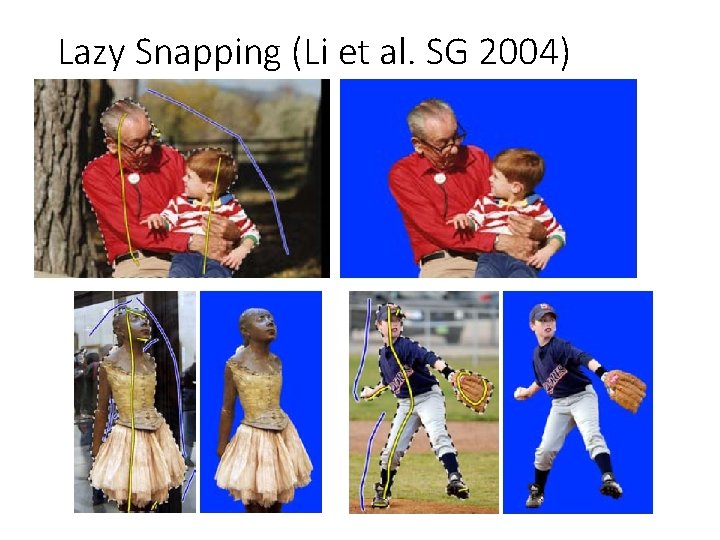
Lazy Snapping (Li et al. SG 2004)

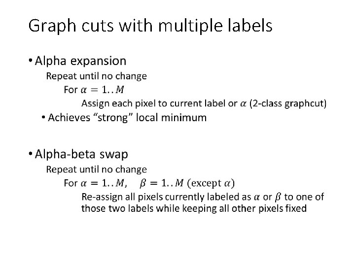
Graph cuts with multiple labels •

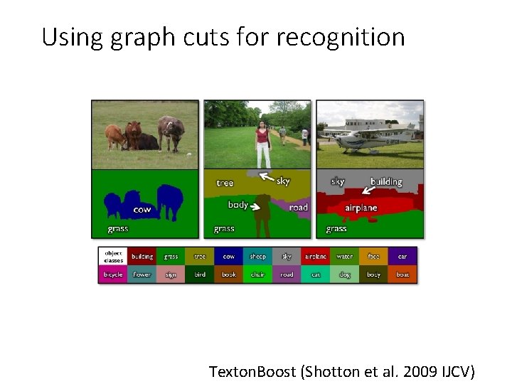
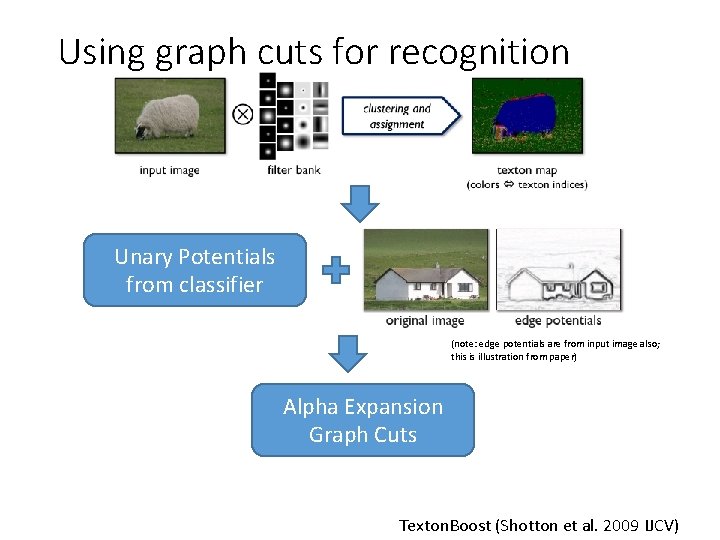
Using graph cuts for recognition Texton. Boost (Shotton et al. 2009 IJCV)

Using graph cuts for recognition Unary Potentials from classifier (note: edge potentials are from input image also; this is illustration from paper) Alpha Expansion Graph Cuts Texton. Boost (Shotton et al. 2009 IJCV)

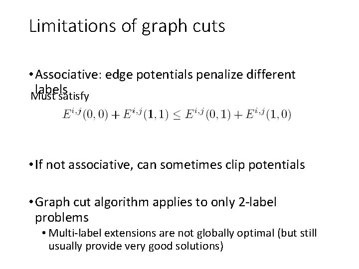
Limitations of graph cuts • Associative: edge potentials penalize different labels Must satisfy • If not associative, can sometimes clip potentials • Graph cut algorithm applies to only 2 -label problems • Multi-label extensions are not globally optimal (but still usually provide very good solutions)

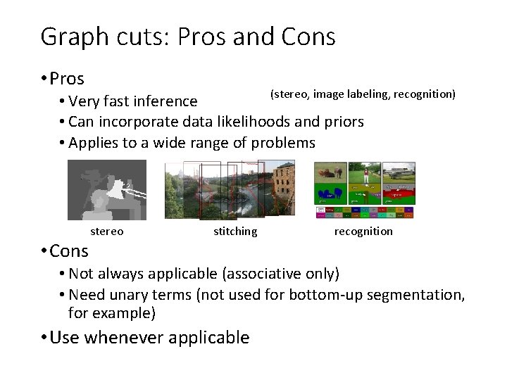
Graph cuts: Pros and Cons • Pros (stereo, image labeling, recognition) • Very fast inference • Can incorporate data likelihoods and priors • Applies to a wide range of problems • Cons stereo stitching recognition • Not always applicable (associative only) • Need unary terms (not used for bottom-up segmentation, for example) • Use whenever applicable

More about MRFs/CRFs • Other common uses • Graph structure on regions • Encoding relations between multiple scene elements • Inference methods • Loopy BP or BP-TRW • Exact for tree-shaped structures • Approximate solutions for general graphs • More widely applicable and can produce marginals but often slower

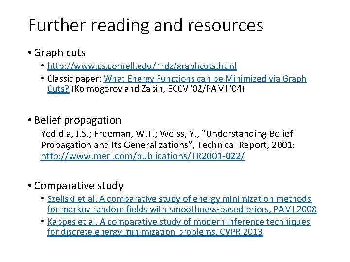
Further reading and resources • Graph cuts • http: //www. cs. cornell. edu/~rdz/graphcuts. html • Classic paper: What Energy Functions can be Minimized via Graph Cuts? (Kolmogorov and Zabih, ECCV '02/PAMI '04) • Belief propagation Yedidia, J. S. ; Freeman, W. T. ; Weiss, Y. , "Understanding Belief Propagation and Its Generalizations”, Technical Report, 2001: http: //www. merl. com/publications/TR 2001 -022/ • Comparative study • Szeliski et al. A comparative study of energy minimization methods for markov random fields with smoothness-based priors, PAMI 2008 • Kappes et al. A comparative study of modern inference techniques for discrete energy minimization problems, CVPR 2013

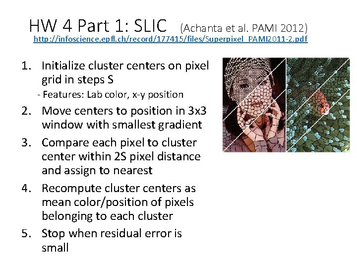
HW 4 Part 1: SLIC (Achanta et al. PAMI 2012) http: //infoscience. epfl. ch/record/177415/files/Superpixel_PAMI 2011 -2. pdf 1. Initialize cluster centers on pixel grid in steps S - Features: Lab color, x-y position 2. Move centers to position in 3 x 3 window with smallest gradient 3. Compare each pixel to cluster center within 2 S pixel distance and assign to nearest 4. Recompute cluster centers as mean color/position of pixels belonging to each cluster 5. Stop when residual error is small

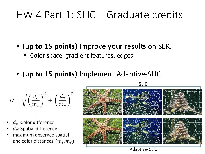
HW 4 Part 1: SLIC – Graduate credits • (up to 15 points) Improve your results on SLIC • Color space, gradient features, edges • (up to 15 points) Implement Adaptive-SLIC

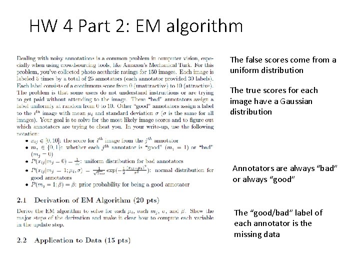
HW 4 Part 2: EM algorithm The false scores come from a uniform distribution The true scores for each image have a Gaussian distribution Annotators are always “bad” or always “good” The “good/bad” label of each annotator is the missing data

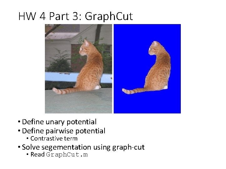
HW 4 Part 3: Graph. Cut • Define unary potential • Define pairwise potential • Contrastive term • Solve segementation using graph-cut • Read Graph. Cut. m

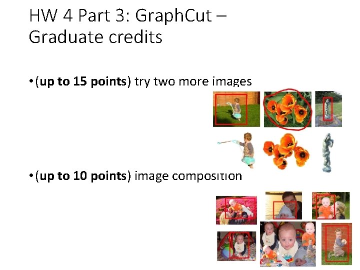
HW 4 Part 3: Graph. Cut – Graduate credits • (up to 15 points) try two more images • (up to 10 points) image composition

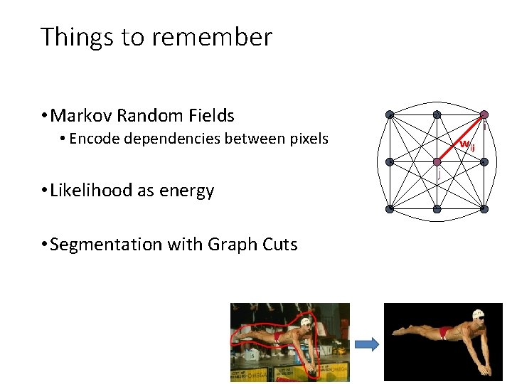
Things to remember • Markov Random Fields • Encode dependencies between pixels • Likelihood as energy • Segmentation with Graph Cuts wij j i

Next module: Object Recognition • Face recognition • Image categorization • Machine learning • Object category detection • Tracking objects