4 1 Modeling and Analysis of Computer Networks

4 -1 Modeling and Analysis of Computer Networks Markov Chains

4 -2 Topics Markov Chains n Discrete-Time Markov Chains n Calculating Stationary Distribution n Global Balance Equations n Detailed Balance Equations n Birth-Death Process n Generalized Markov Chains n Continuous-Time Markov Chains n

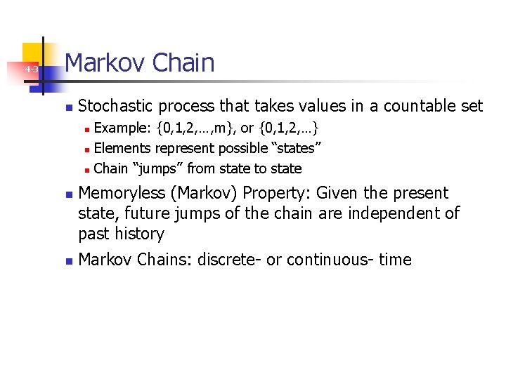
4 -3 Markov Chain n Stochastic process that takes values in a countable set Example: {0, 1, 2, …, m}, or {0, 1, 2, …} n Elements represent possible “states” n Chain “jumps” from state to state n n n Memoryless (Markov) Property: Given the present state, future jumps of the chain are independent of past history Markov Chains: discrete- or continuous- time

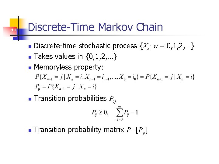
4 -4 Discrete-Time Markov Chain Discrete-time stochastic process {Xn: n = 0, 1, 2, …} n Takes values in {0, 1, 2, …} n Memoryless property: n n Transition probabilities Pij n Transition probability matrix P=[Pij]

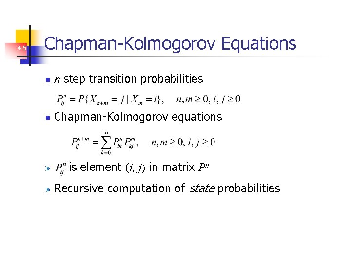
4 -5 Chapman-Kolmogorov Equations n n step transition probabilities n Chapman-Kolmogorov equations is element (i, j) in matrix Pn Recursive computation of state probabilities

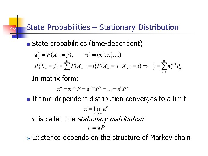
4 -6 State Probabilities – Stationary Distribution n State probabilities (time-dependent) n In matrix form: n If time-dependent distribution converges to a limit n is called the stationary distribution Existence depends on the structure of Markov chain

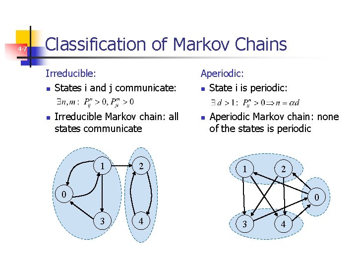
4 -7 Classification of Markov Chains Irreducible: n States i and j communicate: n Irreducible Markov chain: all states communicate 1 2 Aperiodic: n State i is periodic: n Aperiodic Markov chain: none of the states is periodic 1 2 0 0 3 4

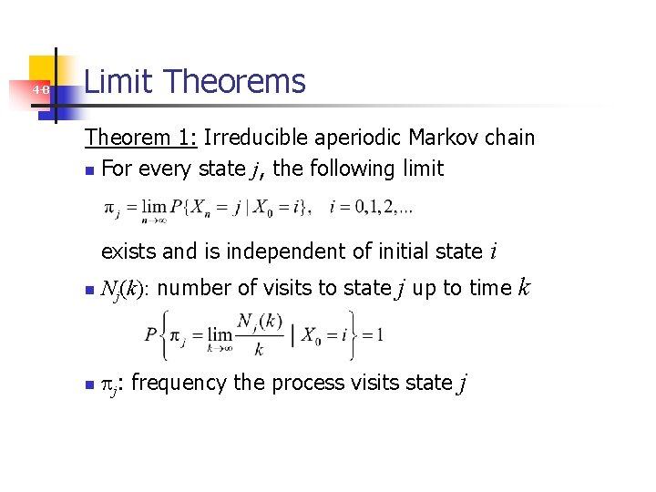
4 -8 Limit Theorems Theorem 1: Irreducible aperiodic Markov chain n For every state j, the following limit exists and is independent of initial state i n Nj(k): number of visits to state j up to time k n j: frequency the process visits state j

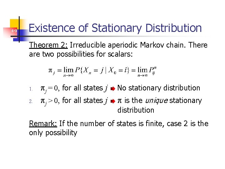
4 -9 Existence of Stationary Distribution Theorem 2: Irreducible aperiodic Markov chain. There are two possibilities for scalars: 1. 2. j = 0, for all states j j > 0, for all states j No stationary distribution is the unique stationary distribution Remark: If the number of states is finite, case 2 is the only possibility

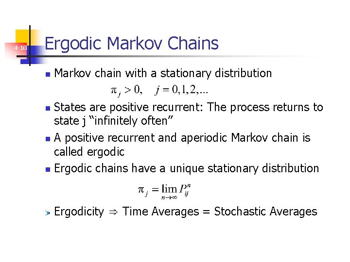
4 -10 Ergodic Markov Chains n Markov chain with a stationary distribution States are positive recurrent: The process returns to state j “infinitely often” n A positive recurrent and aperiodic Markov chain is called ergodic n Ergodic chains have a unique stationary distribution n Ergodicity ⇒ Time Averages = Stochastic Averages

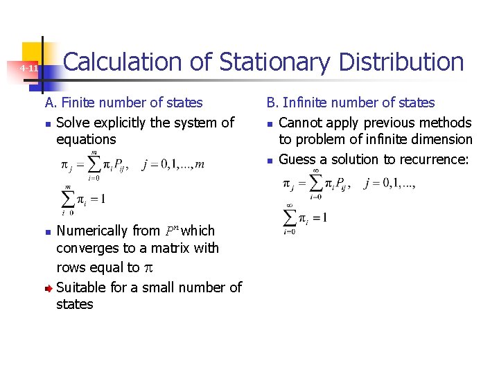
Calculation of Stationary Distribution 4 -11 A. Finite number of states n Solve explicitly the system of equations n Numerically from Pn which converges to a matrix with rows equal to Suitable for a small number of states B. Infinite number of states n Cannot apply previous methods to problem of infinite dimension n Guess a solution to recurrence:

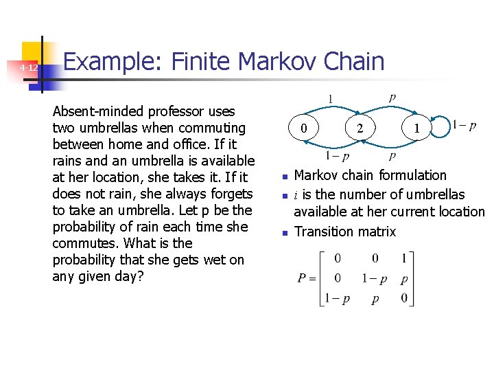
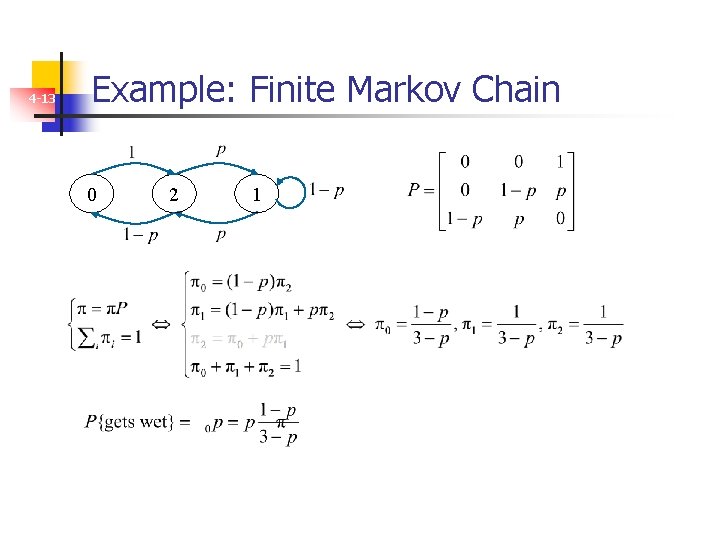
4 -12 Example: Finite Markov Chain Absent-minded professor uses two umbrellas when commuting between home and office. If it rains and an umbrella is available at her location, she takes it. If it does not rain, she always forgets to take an umbrella. Let p be the probability of rain each time she commutes. What is the probability that she gets wet on any given day? 0 n n n 2 1 Markov chain formulation i is the number of umbrellas available at her current location Transition matrix

4 -13 Example: Finite Markov Chain 0 2 1

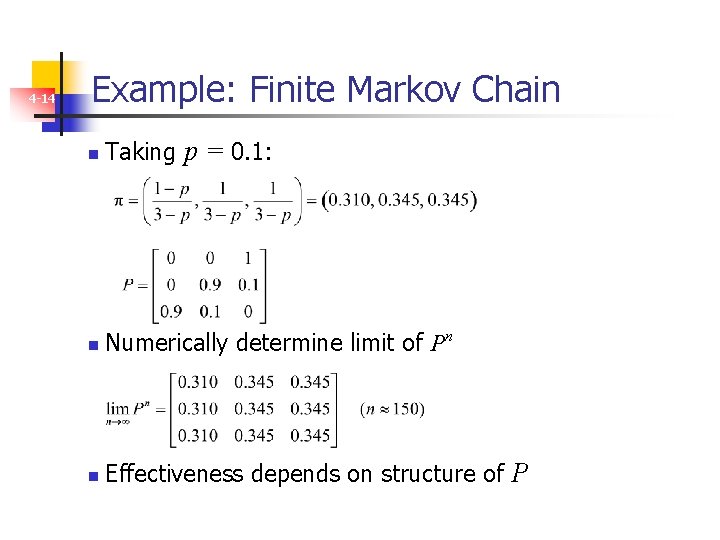
4 -14 Example: Finite Markov Chain n Taking p = 0. 1: n Numerically determine limit of Pn n Effectiveness depends on structure of P

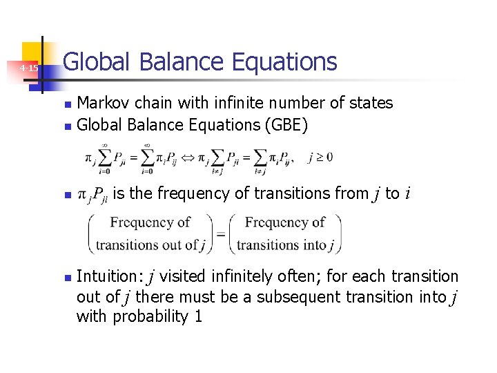
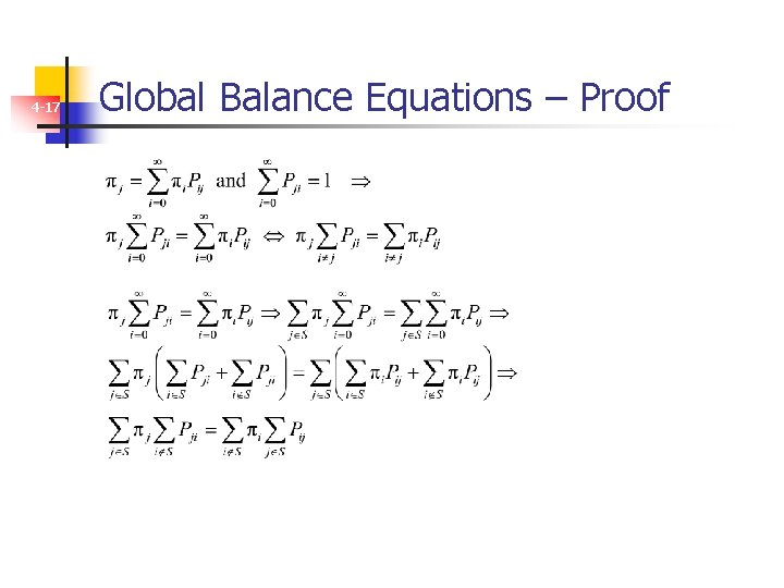
4 -15 Global Balance Equations Markov chain with infinite number of states n Global Balance Equations (GBE) n n n is the frequency of transitions from j to i Intuition: j visited infinitely often; for each transition out of j there must be a subsequent transition into j with probability 1

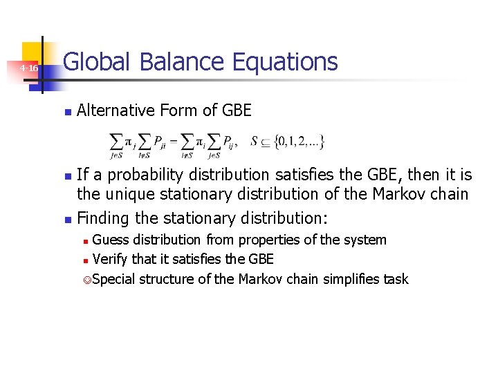
4 -16 Global Balance Equations n Alternative Form of GBE If a probability distribution satisfies the GBE, then it is the unique stationary distribution of the Markov chain n Finding the stationary distribution: n Guess distribution from properties of the system n Verify that it satisfies the GBE J Special structure of the Markov chain simplifies task n

4 -17 Global Balance Equations – Proof

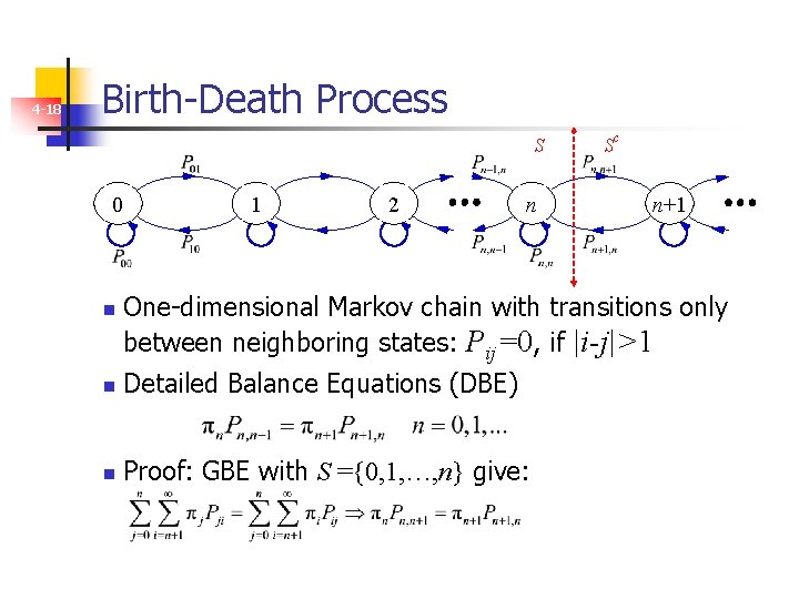
4 -18 Birth-Death Process S 0 n 1 2 n Sc n+1 One-dimensional Markov chain with transitions only between neighboring states: Pij=0, if |i-j|>1 n Detailed Balance Equations (DBE) n Proof: GBE with S ={0, 1, …, n} give:

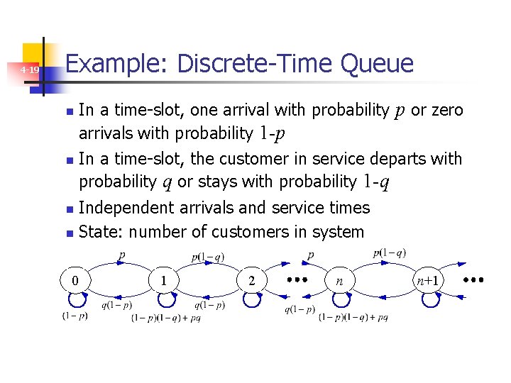
4 -19 Example: Discrete-Time Queue n n In a time-slot, one arrival with probability p or zero arrivals with probability 1 -p In a time-slot, the customer in service departs with probability q or stays with probability 1 -q Independent arrivals and service times n State: number of customers in system n 0 1 2 n n+1

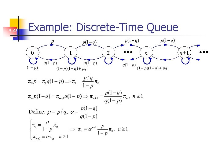
4 -20 Example: Discrete-Time Queue 0 1 2 n n+1

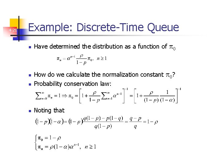
4 -21 Example: Discrete-Time Queue n Have determined the distribution as a function of n How do we calculate the normalization constant Probability conservation law: n Noting that n 0 0?

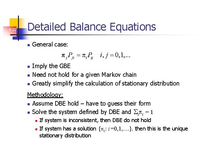
4 -22 Detailed Balance Equations n n General case: Imply the GBE Need not hold for a given Markov chain Greatly simplify the calculation of stationary distribution Methodology: n Assume DBE hold – have to guess their form n Solve the system defined by DBE and i i = 1 n n If system is inconsistent, then DBE do not hold If system has a solution { i: i=0, 1, …}, then this is the unique stationary distribution

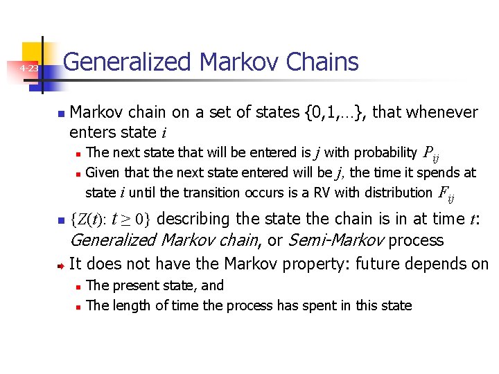
4 -23 Generalized Markov Chains n n Markov chain on a set of states {0, 1, …}, that whenever enters state i n The next state that will be entered is j with probability P ij n Given that the next state entered will be j, the time it spends at state i until the transition occurs is a RV with distribution Fij {Z(t): t ≥ 0} describing the state the chain is in at time t: Generalized Markov chain, or Semi-Markov process It does not have the Markov property: future depends on The present state, and n The length of time the process has spent in this state n

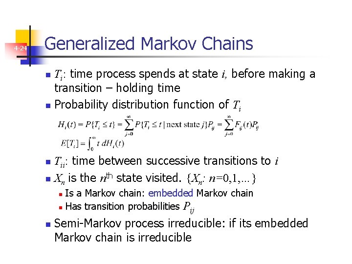
4 -24 Generalized Markov Chains Ti: time process spends at state i, before making a transition – holding time n Probability distribution function of Ti n Tii: time between successive transitions to i n Xn is the nth state visited. {Xn: n=0, 1, …} n Is a Markov chain: embedded Markov chain n Has transition probabilities P ij n n Semi-Markov process irreducible: if its embedded Markov chain is irreducible

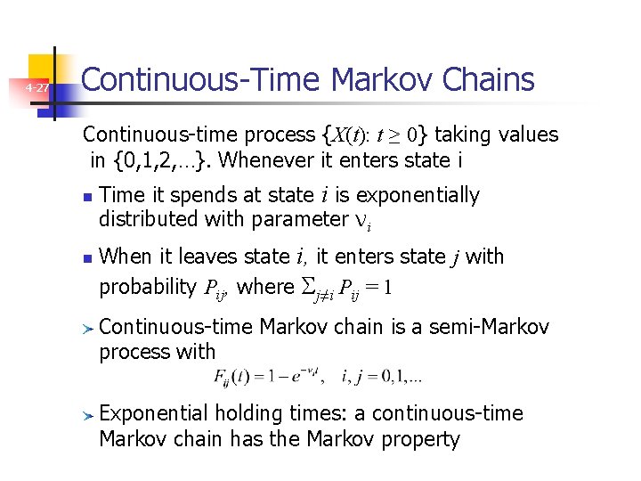
4 -25 Limit Theorems Theorem 3: Irreducible semi-Markov process, E[Tii] < ∞ n For any state j, the following limit exists and is independent of the initial state. n Tj(t): time spent at state j up to time t n pj is equal to the proportion of time spent at state j

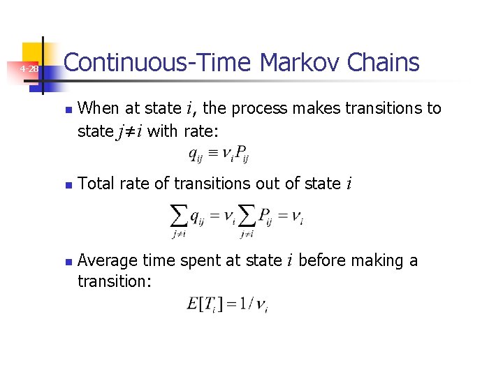
Occupancy Distribution 4 -26 Theorem 4: Irreducible semi-Markov process; E[Tii] < ∞. Embedded Markov chain ergodic; stationary distribution π Occupancy distribution of the semi-Markov process n n πj proportion of transitions into state j E[Tj] mean time spent at j Probability of being at j is proportional to πj. E[Tj]

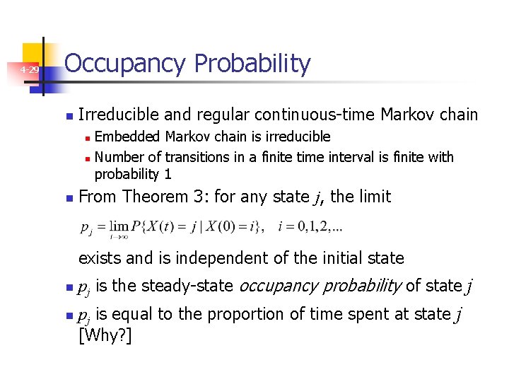
4 -27 Continuous-Time Markov Chains Continuous-time process {X(t): t ≥ 0} taking values in {0, 1, 2, …}. Whenever it enters state i n n Time it spends at state i is exponentially distributed with parameter νi When it leaves state i, it enters state j with probability Pij, where j≠i Pij = 1 Continuous-time Markov chain is a semi-Markov process with Exponential holding times: a continuous-time Markov chain has the Markov property

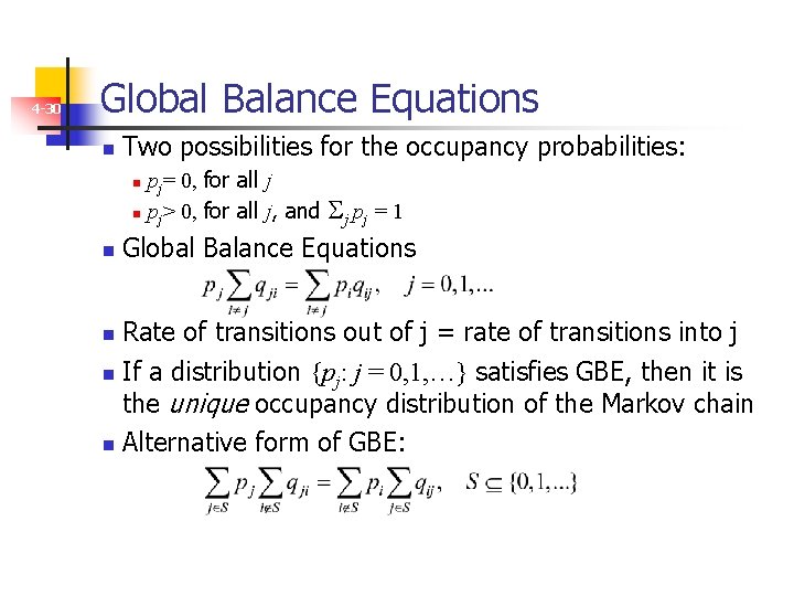
4 -28 Continuous-Time Markov Chains n n n When at state i, the process makes transitions to state j≠i with rate: Total rate of transitions out of state i Average time spent at state i before making a transition:

4 -29 Occupancy Probability n Irreducible and regular continuous-time Markov chain Embedded Markov chain is irreducible n Number of transitions in a finite time interval is finite with probability 1 n n From Theorem 3: for any state j, the limit exists and is independent of the initial state n n pj is the steady-state occupancy probability of state j pj is equal to the proportion of time spent at state j [Why? ]

4 -30 Global Balance Equations n Two possibilities for the occupancy probabilities: pj= 0, for all j n pj> 0, for all j, and n j pj = 1 n Global Balance Equations Rate of transitions out of j = rate of transitions into j n If a distribution {pj: j = 0, 1, …} satisfies GBE, then it is the unique occupancy distribution of the Markov chain n Alternative form of GBE: n

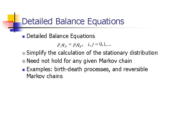
4 -31 Detailed Balance Equations n Detailed Balance Equations Simplify the calculation of the stationary distribution L Need not hold for any given Markov chain n Examples: birth-death processes, and reversible Markov chains J

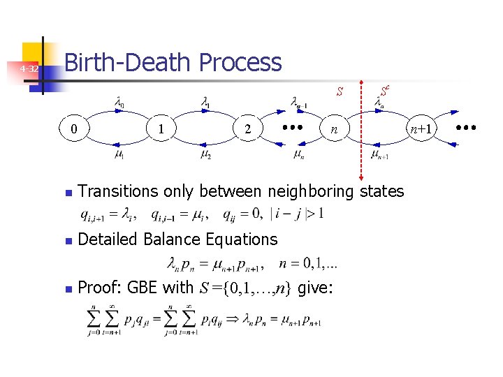
4 -32 Birth-Death Process S 0 1 2 Sc n n Transitions only between neighboring states n Detailed Balance Equations n Proof: GBE with S ={0, 1, …, n} give: n+1

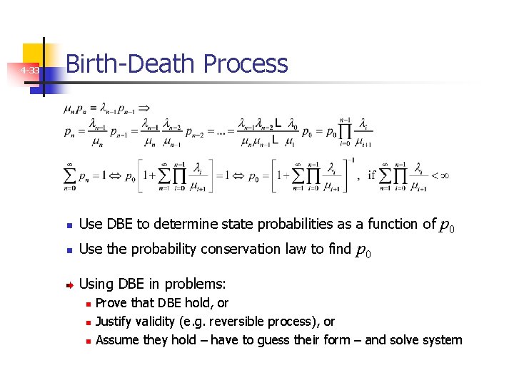
4 -33 Birth-Death Process n Use DBE to determine state probabilities as a function of n Use the probability conservation law to find p 0 Using DBE in problems: n n n Prove that DBE hold, or Justify validity (e. g. reversible process), or Assume they hold – have to guess their form – and solve system

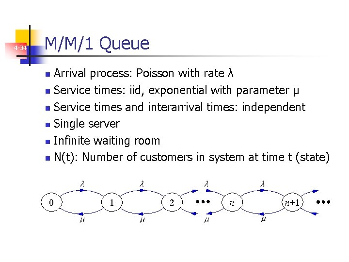
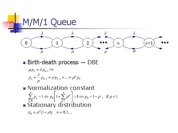
4 -34 M/M/1 Queue Arrival process: Poisson with rate λ n Service times: iid, exponential with parameter µ n Service times and interarrival times: independent n Single server n Infinite waiting room n N(t): Number of customers in system at time t (state) n 0 1 2 n n+1

4 -35 M/M/1 Queue 0 1 2 n Birth-death process → DBE n Normalization constant n Stationary distribution n n+1

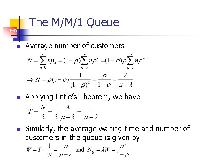
4 -36 The M/M/1 Queue n Average number of customers n Applying Little’s Theorem, we have n Similarly, the average waiting time and number of customers in the queue is given by