A Revealing Introduction to Hidden Markov Models Mark

A Revealing Introduction to Hidden Markov Models Mark Stamp HMM 1

Hidden Markov Models q What is a hidden Markov model (HMM)? u. A machine learning technique u A discrete hill climb technique q Where are HMMs used? u Speech recognition u Malware detection, IDS, etc. q Why is it useful? u Efficient algorithms HMM 2

Markov Chain q Markov chain is a “memoryless random process” q Transitions depend only on u current state and u transition probabilities matrix q Example on next slide… HMM 3

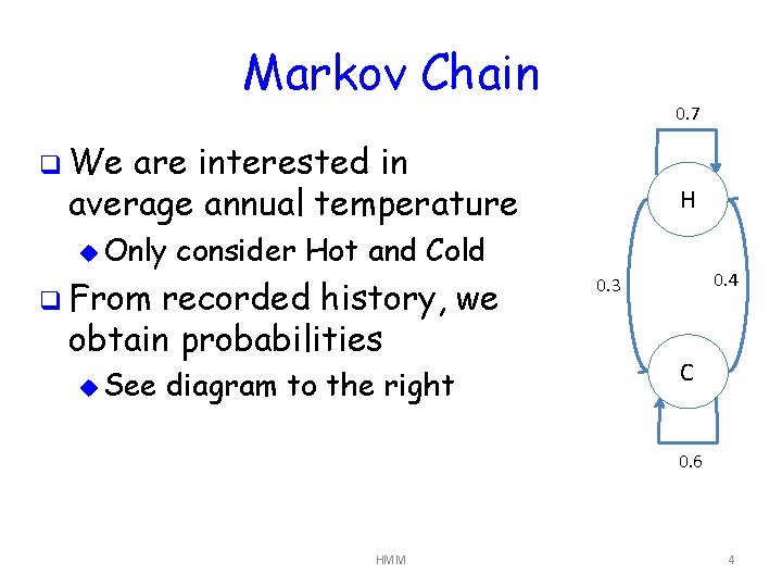
Markov Chain 0. 7 q We are interested in average annual temperature u Only consider Hot and Cold q From recorded history, we obtain probabilities u See H diagram to the right 0. 4 0. 3 C 0. 6 HMM 4

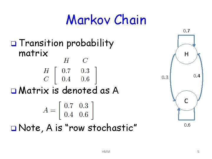
Markov Chain q Transition matrix 0. 7 probability H 0. 4 0. 3 q Matrix q Note, is denoted as A A is “row stochastic” HMM C 0. 6 5

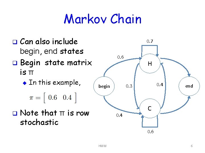
Markov Chain Can also include begin, end states q Begin state matrix is π 0. 7 q u q In this example, 0. 6 0. 4 0. 3 begin Note that π is row stochastic H 0. 4 end C 0. 6 HMM 6

Hidden Markov Model q HMM u But includes a Markov chain this Markov process is “hidden” q Cannot observe the Markov process u Instead, we observe something related to hidden states u It’s as if there is a “curtain” between Markov chain and observations q Example on next slide HMM 7

HMM Example q Consider H/C temperature example q Suppose we want to know H or C temperature in distant past u Before humans (or thermometers) invented u OK if we can just decide Hot versus Cold q We assume transition between Hot and Cold years is same as today u That is, the A matrix is same as today HMM 8

HMM Example q Temp in past determined by Markov process q But, we cannot observe temperature in past q Instead, we note that tree ring size is related to temperature u Look at historical data to see the connection q We u consider 3 tree ring sizes Small, Medium, Large (S, M, L, respectively) q Measure tree ring sizes and recorded temperatures to determine relationship HMM 9

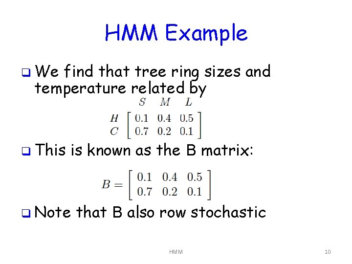
HMM Example q We find that tree ring sizes and temperature related by q This is known as the B matrix: q Note that B also row stochastic HMM 10

HMM Example q Can we now find temps in distant past? q We cannot measure (observe) temp q But we can measure tree ring sizes… q …and tree ring sizes related to temp u By the B matrix q So, we ought to be able to say something about temperature HMM 11

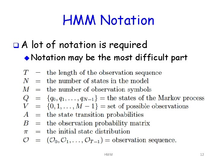
HMM Notation q. A lot of notation is required u Notation may be the most difficult part HMM 12

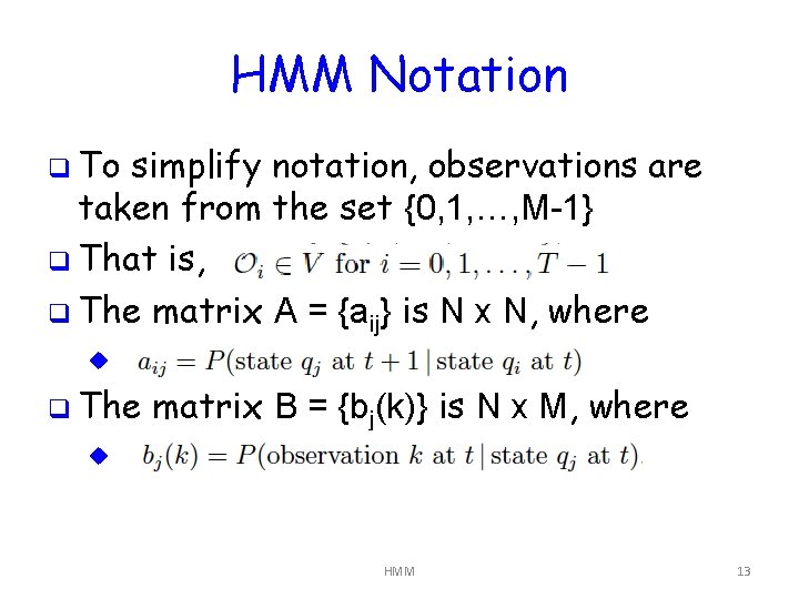
HMM Notation q To simplify notation, observations are taken from the set {0, 1, …, M-1} q That is, q The matrix A = {aij} is N x N, where u q The matrix B = {bj(k)} is N x M, where u HMM 13

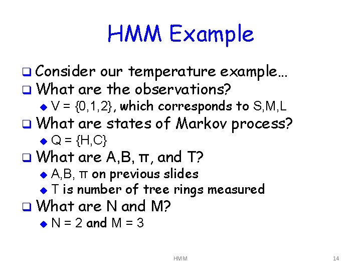
HMM Example q Consider our temperature example… q What are the observations? u V = {0, 1, 2}, which corresponds to S, M, L u Q = {H, C} q What are states of Markov process? are A, B, π, and T? A, B, π on previous slides u T is number of tree rings measured u q What u are N and M? N = 2 and M = 3 HMM 14

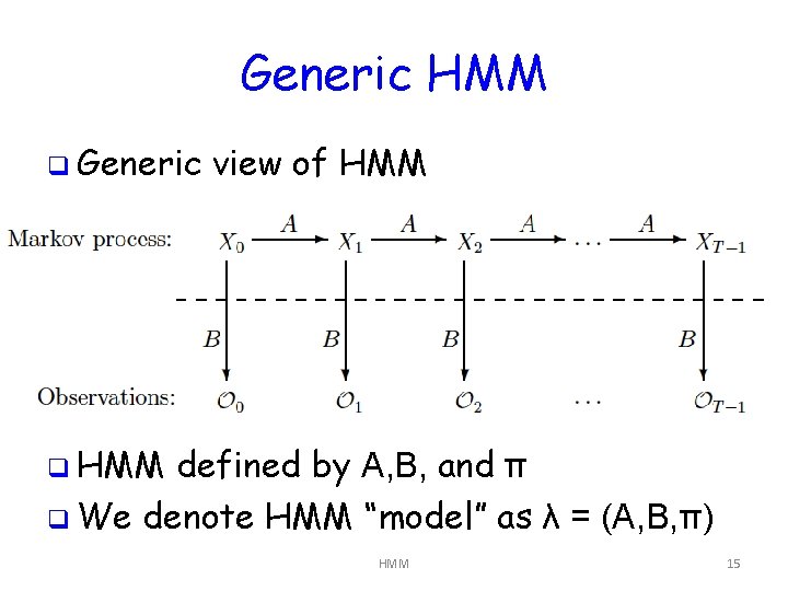
Generic HMM q Generic view of HMM q HMM defined by A, B, and π q We denote HMM “model” as λ = (A, B, π) HMM 15

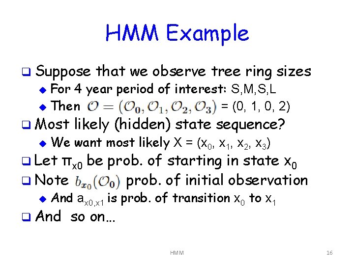
HMM Example q Suppose that we observe tree ring sizes For 4 year period of interest: S, M, S, L u Then = (0, 1, 0, 2) u q Most u likely (hidden) state sequence? We want most likely X = (x 0, x 1, x 2, x 3) q Let πx 0 be prob. of starting in state x 0 q Note prob. of initial observation u And ax 0, x 1 is prob. of transition x 0 to x 1 q And so on… HMM 16

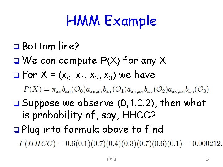
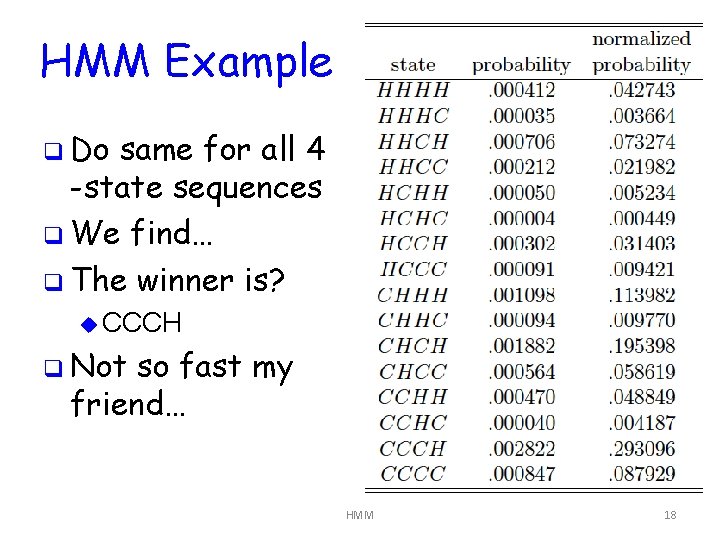
HMM Example q Bottom line? q We can compute P(X) for any X q For X = (x 0, x 1, x 2, x 3) we have q Suppose we observe (0, 1, 0, 2), then what is probability of, say, HHCC? q Plug into formula above to find HMM 17

HMM Example q Do same for all 4 -state sequences q We find… q The winner is? u CCCH q Not so fast my friend… HMM 18

HMM Example q The path CCCH scores the highest q In dynamic programming (DP), we find highest scoring path q But, HMM maximizes expected number of correct states u Sometimes called “EM algorithm” u For “Expectation Maximization” q How does HMM work in this example? HMM 19

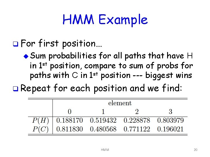
HMM Example q For first position… u Sum probabilities for all paths that have H in 1 st position, compare to sum of probs for paths with C in 1 st position --- biggest wins q Repeat for each position and we find: HMM 20

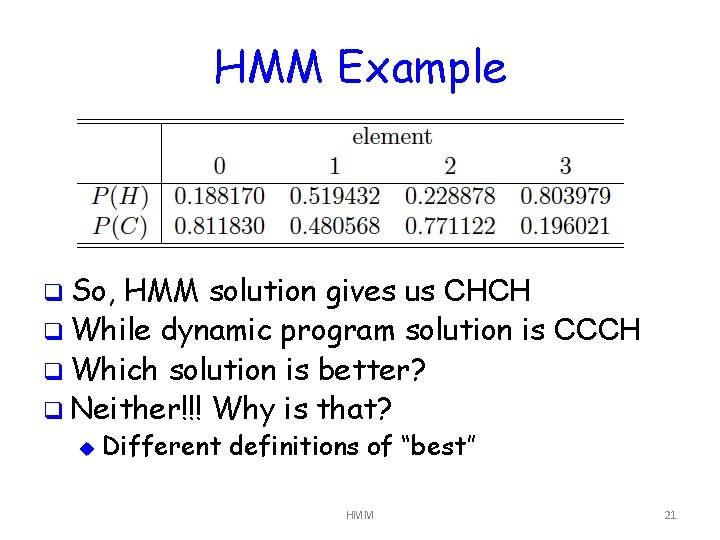
HMM Example q So, HMM solution gives us CHCH q While dynamic program solution is CCCH q Which solution is better? q Neither!!! Why is that? u Different definitions of “best” HMM 21

HMM Paradox? q HMM maximizes expected number of correct states u Whereas q Possible DP chooses “best” overall path for HMM to choose “path” that is impossible u Could q Cannot be a transition probability of 0 get impossible path with DP q Is this a flaw with HMM? u No, it’s a feature… HMM 22

The Three Problems q HMMs used to solve 3 problems q Problem 1: Given a model λ = (A, B, π) and observation sequence O, find P(O|λ) u That is, we score an observation sequence to see how well it fits the given model q Problem 2: Given λ = (A, B, π) and O, find an optimal state sequence u Uncover hidden part (as in previous example) u That is, train a model to fit the observations q Problem 3: Given O, N, and M, find the model λ that maximizes probability of O HMM 23

HMMs in Practice q Typically, HMMs used as follows q Given an observation sequence q Assume a hidden Markov process exists q Train a model based on observations u Problem q Then 3 (determine N by trial and error) given a sequence of observations, score it vs model from previous step u Problem 1 (high score implies it’s similar to training data) HMM 24

HMMs in Practice q Previous slide gives sense in which HMM is a “machine learning” technique u We do not need to specify anything except the parameter N u And “best” N found by trial and error q That is, we don’t have to think too much u Just train HMM and then use it u Best of all, efficient algorithms for HMMs HMM 25

The Three Solutions q We give detailed solutions to the three problems q Note: We must have efficient solutions q Recall the three problems: Problem 1: Score an observation sequence versus a given model u Problem 2: Given a model, “uncover” hidden part u Problem 3: Given an observation sequence, train a model u HMM 26

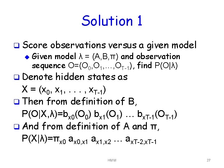
Solution 1 q Score u observations versus a given model Given model λ = (A, B, π) and observation sequence O=(O 0, O 1, …, OT-1), find P(O|λ) q Denote hidden states as X = (x 0, x 1, . . . , x. T-1) q Then from definition of B, P(O|X, λ)=bx 0(O 0) bx 1(O 1) … bx. T-1(OT-1) q And from definition of A and π, P(X|λ)=πx 0 ax 0, x 1 ax 1, x 2 … ax. T-2, x. T-1 HMM 27

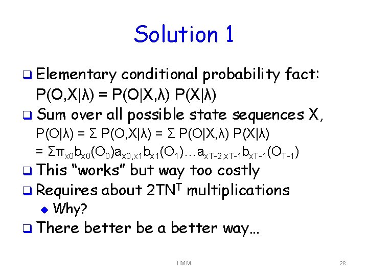
Solution 1 q Elementary conditional probability fact: P(O, X|λ) = P(O|X, λ) P(X|λ) q Sum over all possible state sequences X, P(O|λ) = Σ P(O, X|λ) = Σ P(O|X, λ) P(X|λ) = Σπx 0 bx 0(O 0)ax 0, x 1 bx 1(O 1)…ax. T-2, x. T-1 bx. T-1(OT-1) q This “works” but way too costly q Requires about 2 TNT multiplications u Why? q There better be a better way… HMM 28

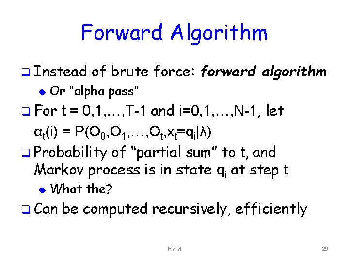
Forward Algorithm q Instead u of brute force: forward algorithm Or “alpha pass” q For t = 0, 1, …, T-1 and i=0, 1, …, N-1, let αt(i) = P(O 0, O 1, …, Ot, xt=qi|λ) q Probability of “partial sum” to t, and Markov process is in state qi at step t u What the? q Can be computed recursively, efficiently HMM 29

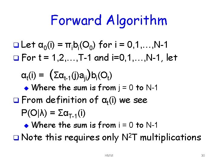
Forward Algorithm q Let α 0(i) = πibi(O 0) for i = 0, 1, …, N-1 q For t = 1, 2, …, T-1 and i=0, 1, …, N-1, let αt(i) = u (Σαt-1(j)aji)bi(Ot) Where the sum is from j = 0 to N-1 q From definition of αt(i) we see P(O|λ) = ΣαT-1(i) u Where the sum is from i = 0 to N-1 q Note this requires only N 2 T multiplications HMM 30

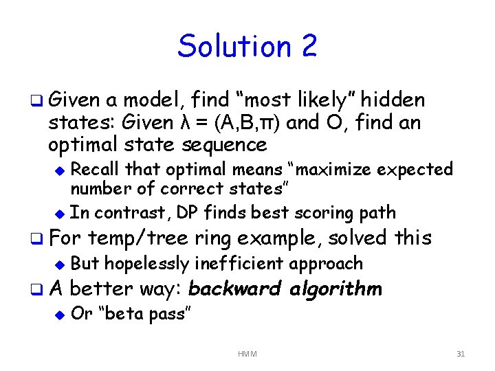
Solution 2 q Given a model, find “most likely” hidden states: Given λ = (A, B, π) and O, find an optimal state sequence Recall that optimal means “maximize expected number of correct states” u In contrast, DP finds best scoring path u q For u q. A u temp/tree ring example, solved this But hopelessly inefficient approach better way: backward algorithm Or “beta pass” HMM 31

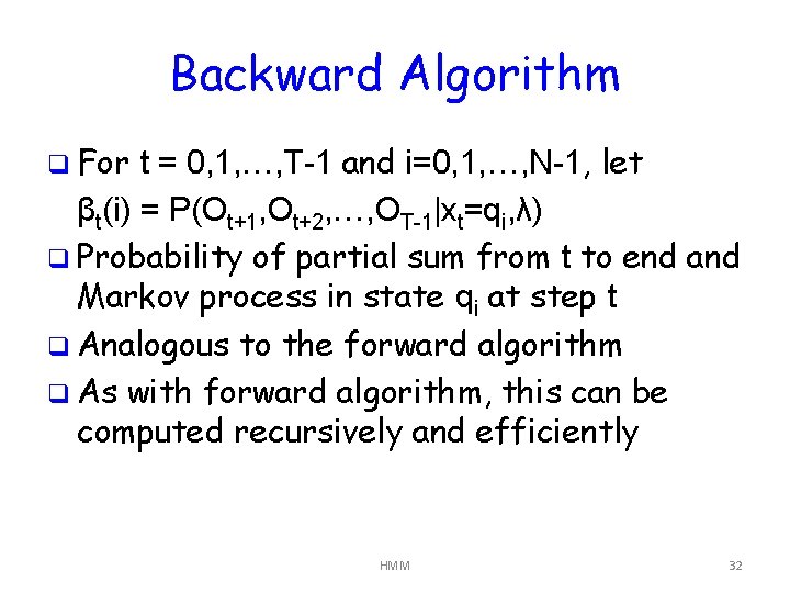
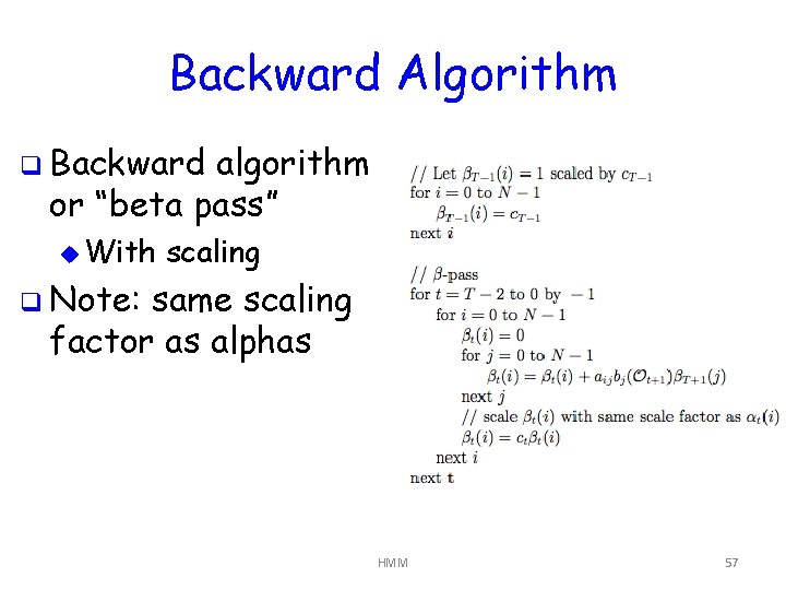
Backward Algorithm q For t = 0, 1, …, T-1 and i=0, 1, …, N-1, let βt(i) = P(Ot+1, Ot+2, …, OT-1|xt=qi, λ) q Probability of partial sum from t to end and Markov process in state qi at step t q Analogous to the forward algorithm q As with forward algorithm, this can be computed recursively and efficiently HMM 32

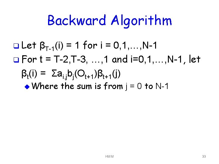
Backward Algorithm q Let βT-1(i) = 1 for i = 0, 1, …, N-1 q For t = T-2, T-3, …, 1 and i=0, 1, …, N-1, let βt(i) = Σai, jbj(Ot+1)βt+1(j) u Where the sum is from j = 0 to N-1 HMM 33

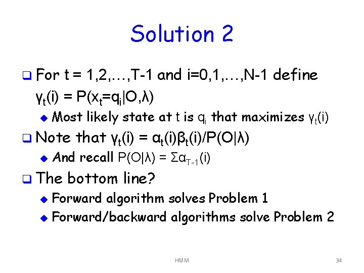
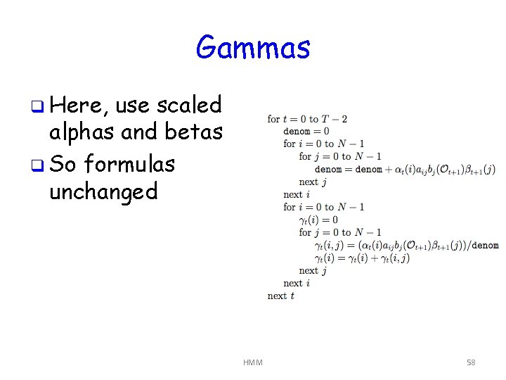
Solution 2 q For t = 1, 2, …, T-1 and i=0, 1, …, N-1 define γt(i) = P(xt=qi|O, λ) u Most likely state at t is qi that maximizes γt(i) q Note u that γt(i) = αt(i)βt(i)/P(O|λ) And recall P(O|λ) = ΣαT-1(i) q The bottom line? Forward algorithm solves Problem 1 u Forward/backward algorithms solve Problem 2 u HMM 34

Solution 3 q Train a model: Given O, N, and M, find λ that maximizes probability of O q Here, we iteratively adjust λ = (A, B, π) to better fit the given observations O u The size of matrices are fixed (N and M) u But elements of matrices can change q It is amazing that this works! u And even more amazing that it’s efficient HMM 35

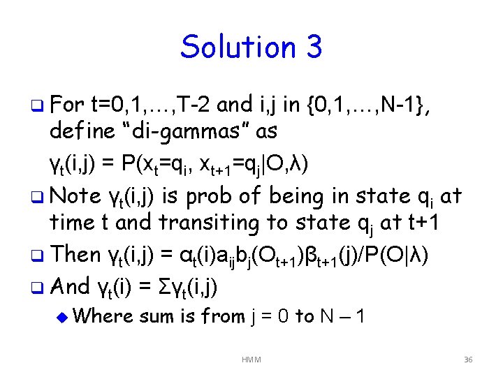
Solution 3 q For t=0, 1, …, T-2 and i, j in {0, 1, …, N-1}, define “di-gammas” as γt(i, j) = P(xt=qi, xt+1=qj|O, λ) q Note γt(i, j) is prob of being in state qi at time t and transiting to state qj at t+1 q Then γt(i, j) = αt(i)aijbj(Ot+1)βt+1(j)/P(O|λ) q And γt(i) = Σγt(i, j) u Where sum is from j = 0 to N – 1 HMM 36

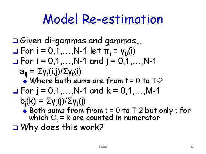
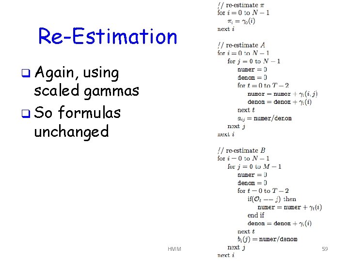
Model Re-estimation q Given di-gammas and gammas… q For i = 0, 1, …, N-1 let πi = γ 0(i) q For i = 0, 1, …, N-1 and j = 0, 1, …, N-1 aij = Σγt(i, j)/Σγt(i) u Where both sums are from t = 0 to T-2 q For j = 0, 1, …, N-1 and k = 0, 1, …, M-1 bj(k) = Σγt(j)/Σγt(j) u Both sums from t = 0 to T-2 but only t for which Ot = k are counted in numerator q Why does this work? HMM 37

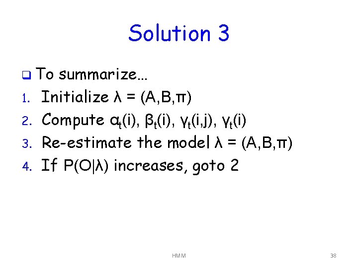
Solution 3 q To 1. 2. 3. 4. summarize… Initialize λ = (A, B, π) Compute αt(i), βt(i), γt(i, j), γt(i) Re-estimate the model λ = (A, B, π) If P(O|λ) increases, goto 2 HMM 38

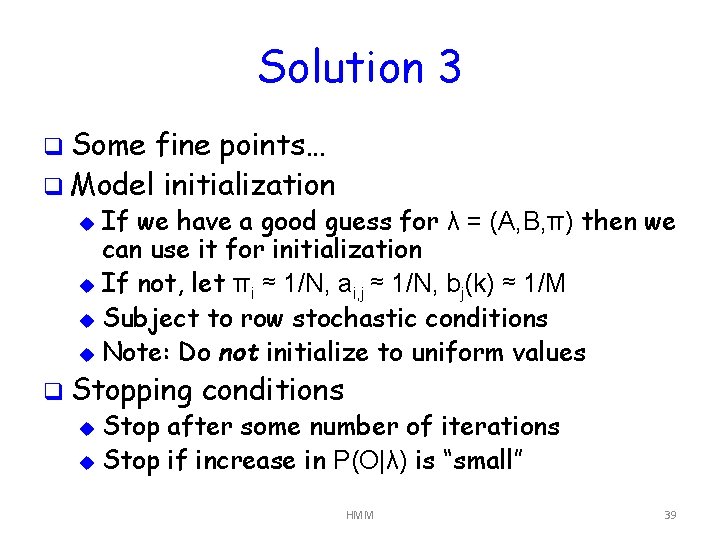
Solution 3 q Some fine points… q Model initialization If we have a good guess for λ = (A, B, π) then we can use it for initialization u If not, let πi ≈ 1/N, ai, j ≈ 1/N, bj(k) ≈ 1/M u Subject to row stochastic conditions u Note: Do not initialize to uniform values u q Stopping conditions Stop after some number of iterations u Stop if increase in P(O|λ) is “small” u HMM 39

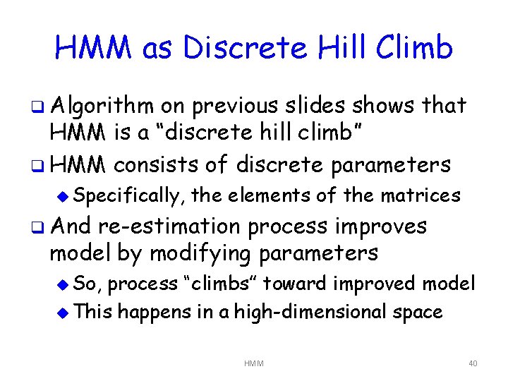
HMM as Discrete Hill Climb q Algorithm on previous slides shows that HMM is a “discrete hill climb” q HMM consists of discrete parameters u Specifically, the elements of the matrices q And re-estimation process improves model by modifying parameters u So, process “climbs” toward improved model u This happens in a high-dimensional space HMM 40

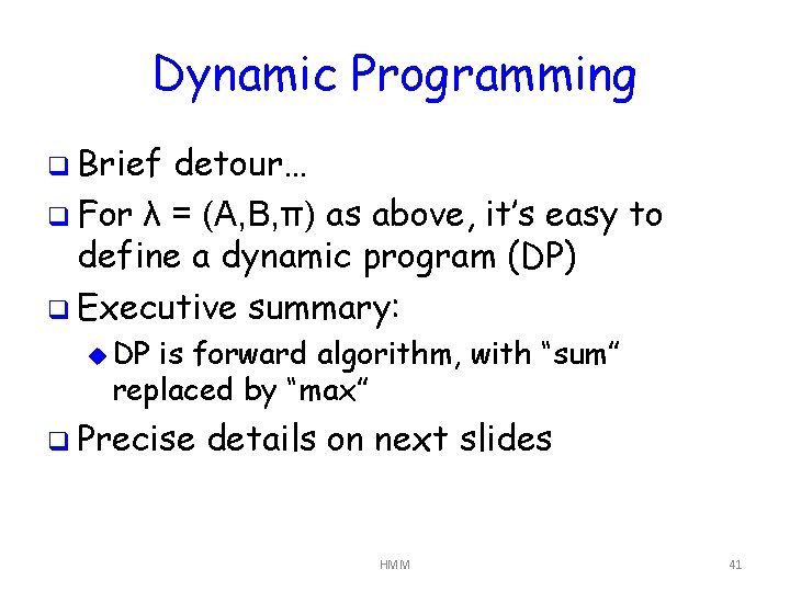
Dynamic Programming q Brief detour… q For λ = (A, B, π) as above, it’s easy to define a dynamic program (DP) q Executive summary: u DP is forward algorithm, with “sum” replaced by “max” q Precise details on next slides HMM 41

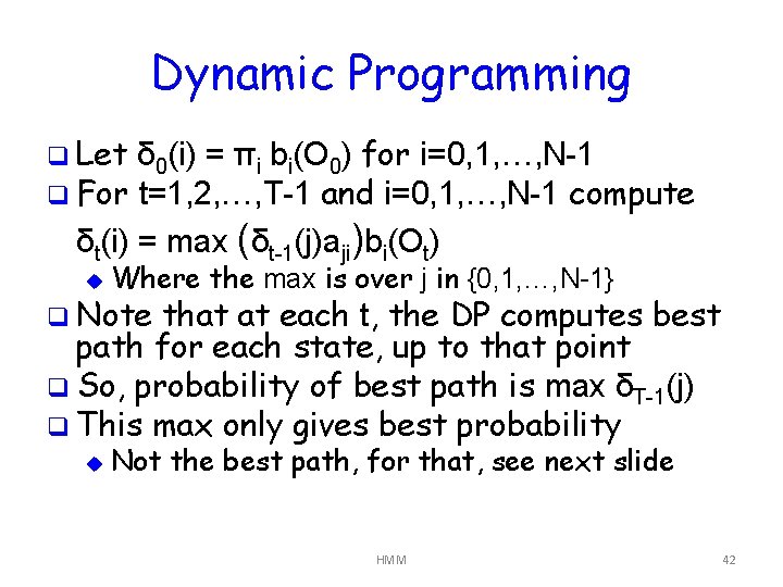
Dynamic Programming q Let δ 0(i) = πi bi(O 0) for i=0, 1, …, N-1 q For t=1, 2, …, T-1 and i=0, 1, …, N-1 compute δt(i) = max (δt-1(j)aji)bi(Ot) u Where the max is over j in {0, 1, …, N-1} u Not the best path, for that, see next slide q Note that at each t, the DP computes best path for each state, up to that point q So, probability of best path is max δT-1(j) q This max only gives best probability HMM 42

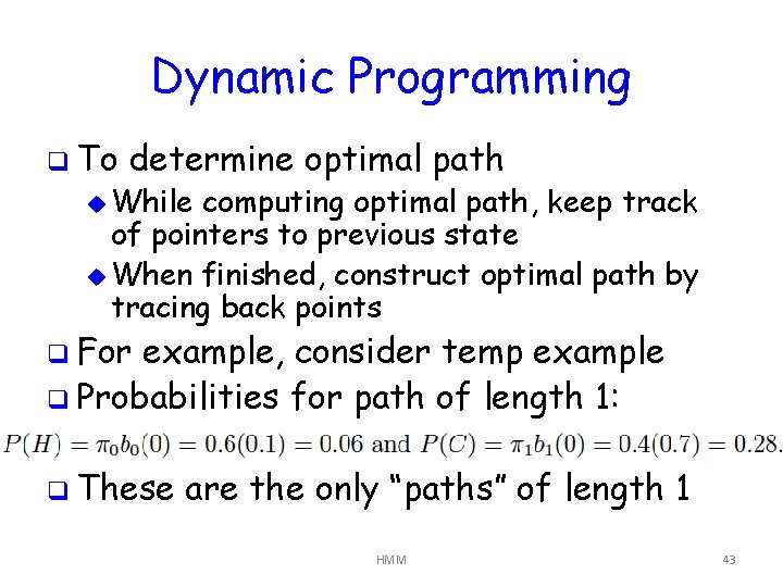
Dynamic Programming q To determine optimal path u While computing optimal path, keep track of pointers to previous state u When finished, construct optimal path by tracing back points q For example, consider temp example q Probabilities for path of length 1: q These are the only “paths” of length 1 HMM 43

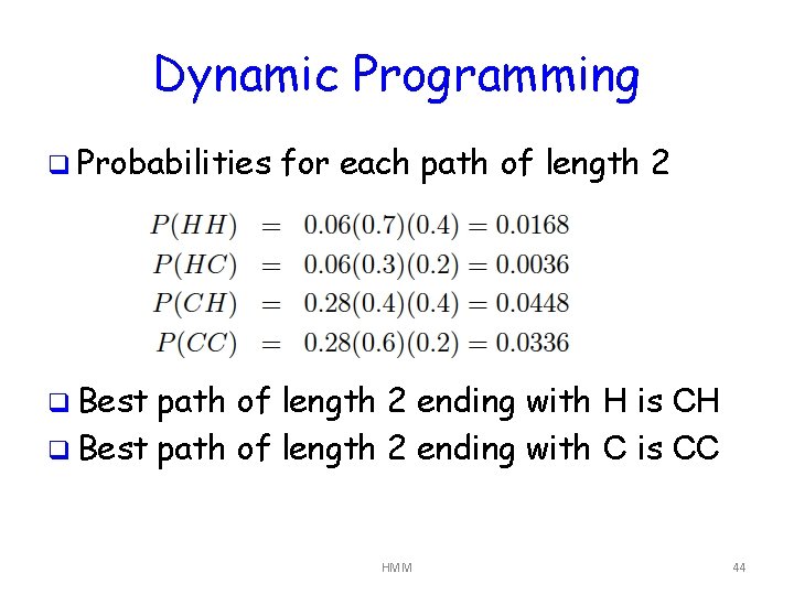
Dynamic Programming q Probabilities for each path of length 2 q Best path of length 2 ending with H is CH q Best path of length 2 ending with C is CC HMM 44

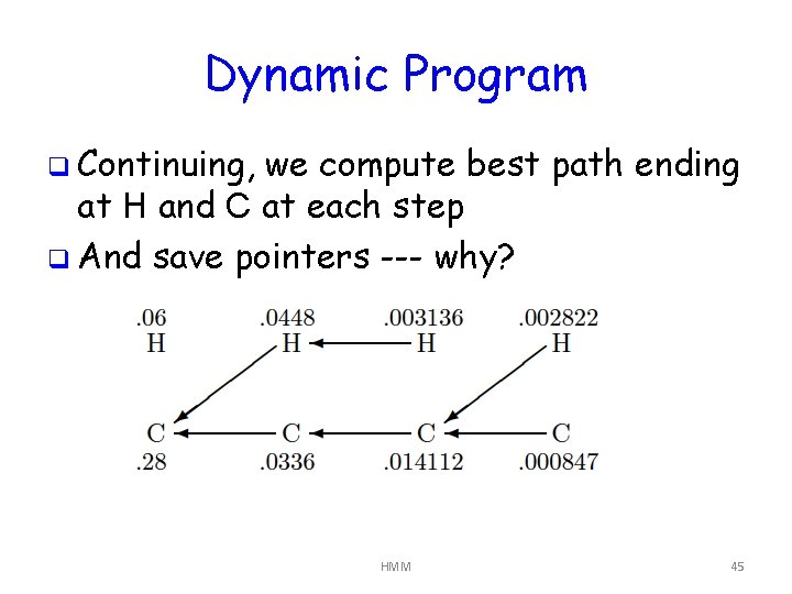
Dynamic Program q Continuing, we compute best path ending at H and C at each step q And save pointers --- why? HMM 45

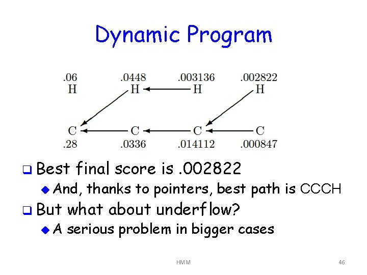
Dynamic Program q Best final score is. 002822 u And, q But u. A thanks to pointers, best path is CCCH what about underflow? serious problem in bigger cases HMM 46

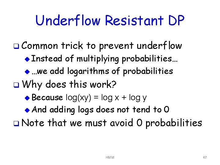
Underflow Resistant DP q Common trick to prevent underflow u Instead of multiplying probabilities… u …we add logarithms of probabilities q Why does this work? u Because log(xy) = log x + log y u And adding logs does not tend to 0 q Note that we must avoid 0 probabilities HMM 47

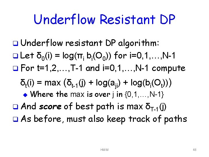
Underflow Resistant DP q Underflow resistant DP algorithm: q Let δ 0(i) = log(πi bi(O 0)) for i=0, 1, …, N-1 q For t=1, 2, …, T-1 and i=0, 1, …, N-1 compute δt(i) = max (δt-1(j) + log(aji) + log(bi(Ot))) u Where the max is over j in {0, 1, …, N-1} q And score of best path is max δT-1(j) q As before, must also keep track of paths HMM 48

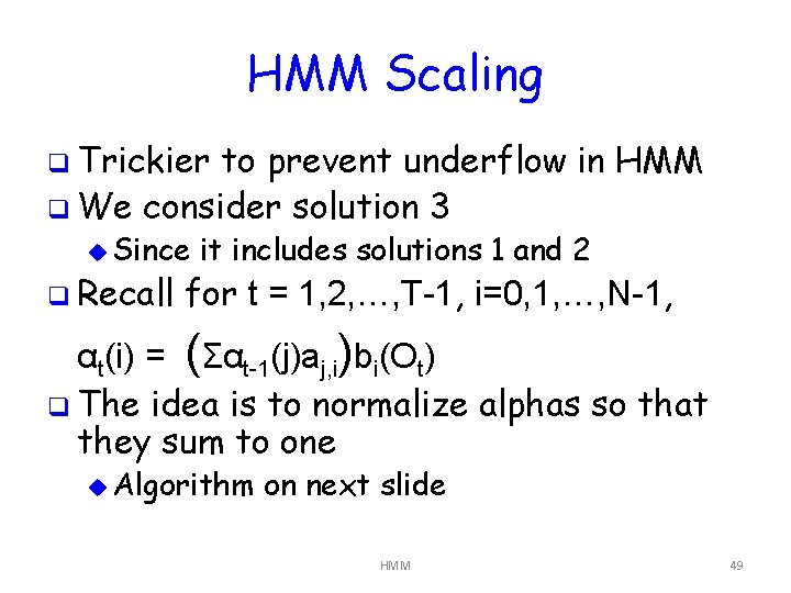
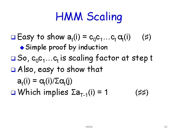
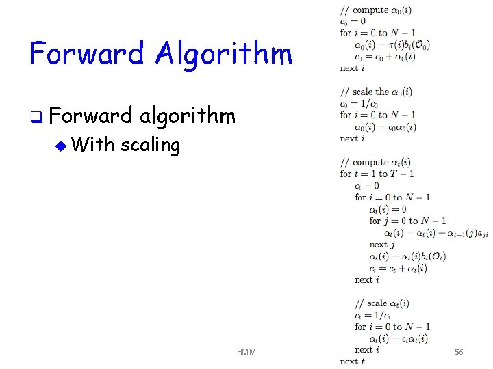
HMM Scaling q Trickier to prevent underflow in HMM q We consider solution 3 u Since q Recall it includes solutions 1 and 2 for t = 1, 2, …, T-1, i=0, 1, …, N-1, αt(i) = (Σαt-1(j)aj, i)bi(Ot) q The idea is to normalize alphas so that they sum to one u Algorithm on next slide HMM 49

HMM Scaling q Given αt(i) = (Σαt-1(j)aj, i)bi(Ot) q Let a 0(i) = α 0(i) for i=0, 1, …, N-1 q Let c 0 = 1/Σa 0(j) q For i = 0, 1, …, N-1, let a 0(i) = c 0 a 0(i) q This takes care of t = 0 case q Algorithm continued on next slide… HMM 50

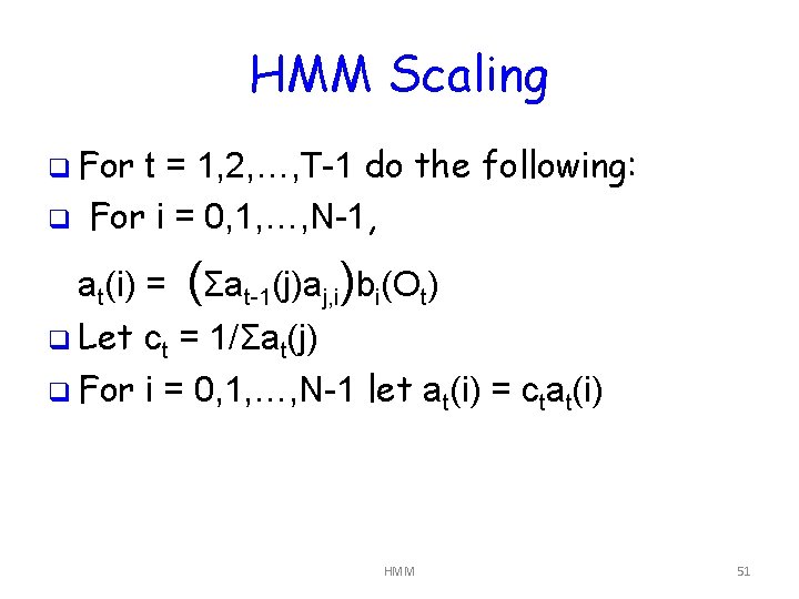
HMM Scaling q For q t = 1, 2, …, T-1 do the following: For i = 0, 1, …, N-1, at(i) = (Σat-1(j)aj, i)bi(Ot) q Let ct = 1/Σat(j) q For i = 0, 1, …, N-1 let at(i) = ctat(i) HMM 51

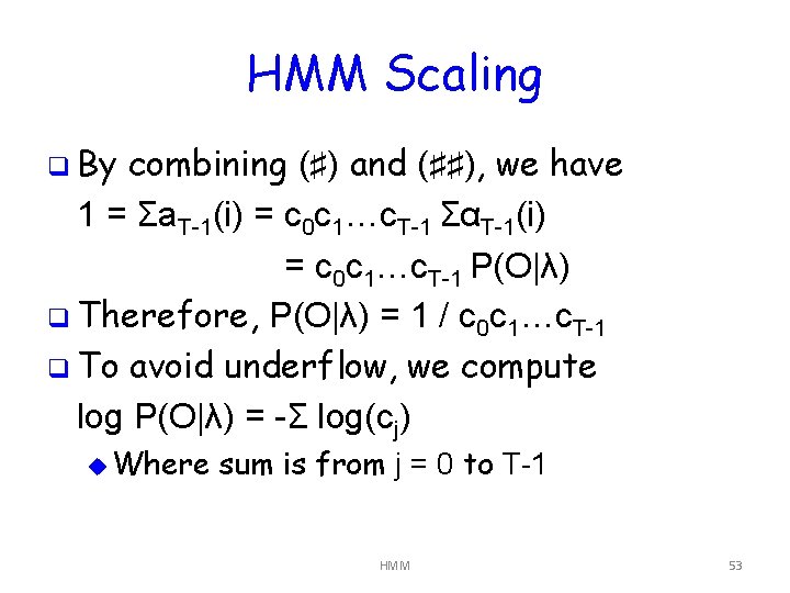
HMM Scaling q Easy to show at(i) = c 0 c 1…ct αt(i) u Simple (♯) proof by induction q So, c 0 c 1…ct is scaling factor at step t q Also, easy to show that at(i) = αt(i)/Σαt(j) q Which implies Σa. T-1(i) = 1 (♯♯) HMM 52

HMM Scaling q By combining (♯) and (♯♯), we have 1 = Σa. T-1(i) = c 0 c 1…c. T-1 ΣαT-1(i) = c 0 c 1…c. T-1 P(O|λ) q Therefore, P(O|λ) = 1 / c 0 c 1…c. T-1 q To avoid underflow, we compute log P(O|λ) = -Σ log(cj) u Where sum is from j = 0 to T-1 HMM 53

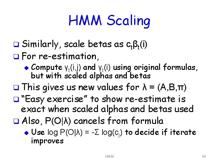
HMM Scaling q Similarly, scale betas as ctβt(i) q For re-estimation, u Compute γt(i, j) and γt(i) using original formulas, but with scaled alphas and betas q This gives us new values for λ = (A, B, π) q “Easy exercise” to show re-estimate is exact when scaled alphas and betas used q Also, P(O|λ) cancels from formula u Use log P(O|λ) = -Σ log(cj) to decide if iterate improves HMM 54

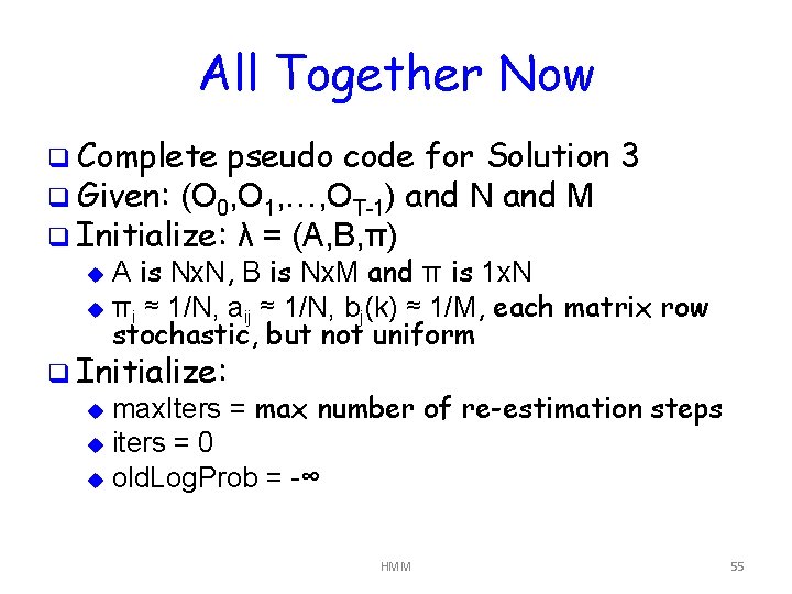
All Together Now q Complete pseudo code for Solution 3 q Given: (O 0, O 1, …, OT-1) and N and M q Initialize: λ = (A, B, π) A is Nx. N, B is Nx. M and π is 1 x. N u πi ≈ 1/N, aij ≈ 1/N, bj(k) ≈ 1/M, each matrix row stochastic, but not uniform u q Initialize: max. Iters = max number of re-estimation steps u iters = 0 u old. Log. Prob = -∞ u HMM 55

Forward Algorithm q Forward u With algorithm scaling HMM 56

Backward Algorithm q Backward algorithm or “beta pass” u With scaling q Note: same scaling factor as alphas HMM 57

Gammas q Here, use scaled alphas and betas q So formulas unchanged HMM 58

Re-Estimation q Again, using scaled gammas q So formulas unchanged HMM 59

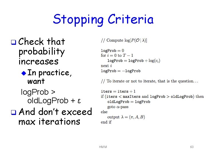
Stopping Criteria q Check that probability increases u In practice, want log. Prob > old. Log. Prob + ε q And don’t exceed max iterations HMM 60

English Text Example q Suppose Martian arrives on earth u Sees written English text u Wants to learn something about it u Martians know about HMMs q So, strip our all non-letters, make all letters lower-case u 27 symbols (letters, plus word-space) u Train HMM on long sequence of symbols HMM 61

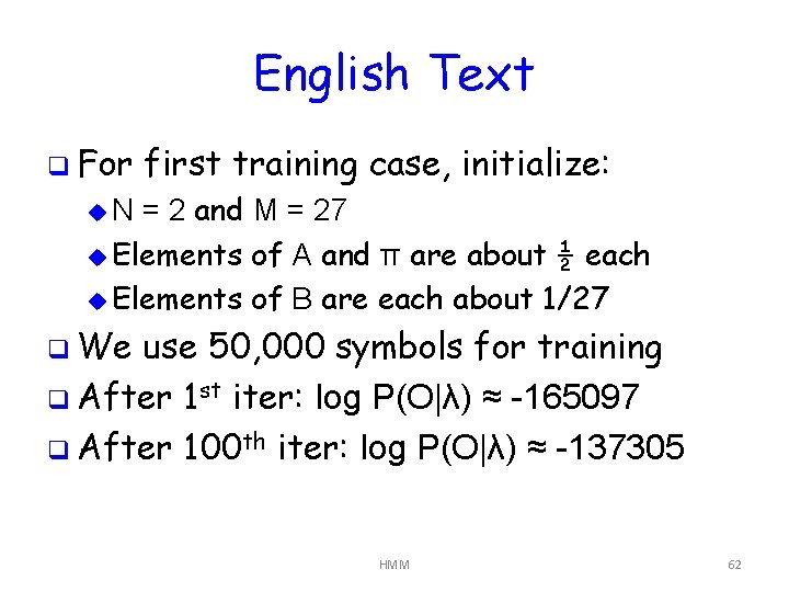
English Text q For first training case, initialize: = 2 and M = 27 u Elements of A and π are about ½ each u Elements of B are each about 1/27 u. N q We use 50, 000 symbols for training q After 1 st iter: log P(O|λ) ≈ -165097 q After 100 th iter: log P(O|λ) ≈ -137305 HMM 62

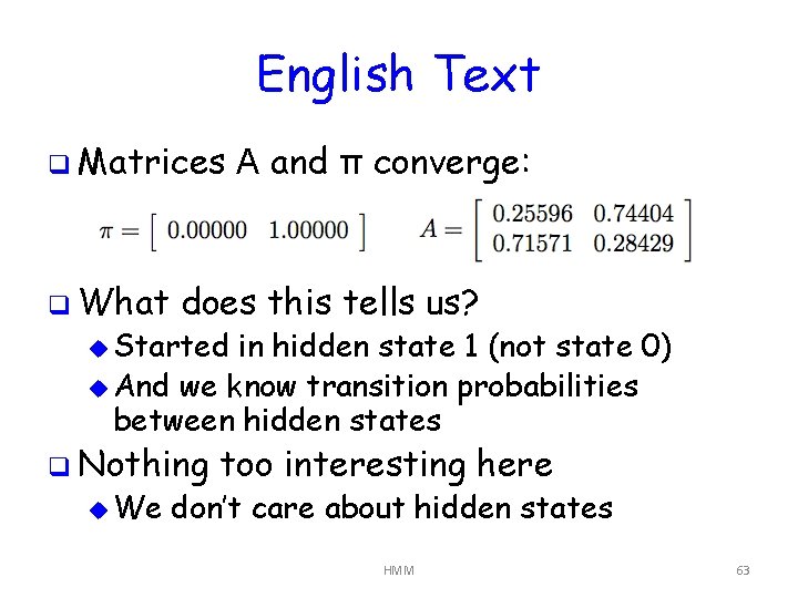
English Text q Matrices q What A and π converge: does this tells us? u Started in hidden state 1 (not state 0) u And we know transition probabilities between hidden states q Nothing u We too interesting here don’t care about hidden states HMM 63

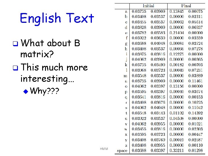
English Text q What about B matrix? q This much more interesting… u Why? ? ? HMM 64

A Security Application q Suppose we want to detect metamorphic computer viruses Such viruses vary their internal structure u But function of malware stays same u If sufficiently variable, standard signature detection will fail u q Can we use HMM for detection? What to use as observation sequence? u Is there really a “hidden” Markov process? u What about N, M, and T? u How many Os needed for training, scoring? u HMM 65

HMM for Metamorphic Detection q Set of “family” viruses into 2 subsets q Extract opcodes from each virus q Append opcodes from subset 1 to make one long sequence Train HMM on opcode sequence (problem 3) u Obtain a model λ = (A, B, π) u q Set threshold: score opcodes from files in subset 2 and “normal” files (problem 1) Can you sets a threshold that separates sets? u If so, may have a viable detection method u HMM 66

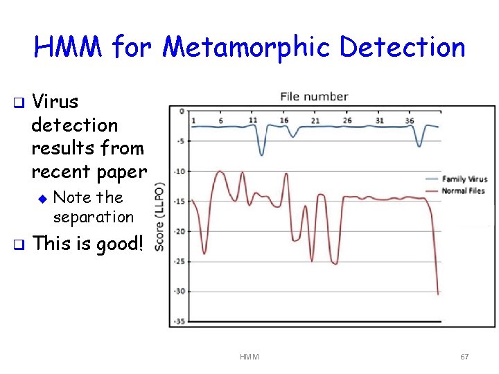
HMM for Metamorphic Detection q Virus detection results from recent paper u q Note the separation This is good! HMM 67

HMM Generalizations q Here, u assumed Markov process of order 1 Current state depends only on previous state and transition matrix q Can use higher order Markov process Current state depends on n previous states u Higher order vs increased N ? u q Can have A and B matrices depend on t q HMM often combined with other techniques (e. g. , neural nets) HMM 68

Generalizations q In some cases, big limitation of HMM is that position information is not used u In many applications this is OK/desirable u In some apps, this is a serious limitation q Bioinformatics u DNA applications sequencing, protein alignment, etc. u Sequence alignment is crucial u They use “profile HMMs” instead of HMMs u PHMM is next topic… HMM 69

References q. A revealing introduction to hidden Markov models, by M. Stamp u http: //www. cs. sjsu. edu/faculty/stamp/RU A/HMM. pdf q. A tutorial on hidden Markov models and selected applications in speech recognition, by L. R. Rabiner u http: //www. cs. ubc. ca/~murphyk/Bayes/rab iner. pdf HMM 70

References q Hunting for metamorphic engines, W. Wong and M. Stamp u Journal in Computer Virology, Vol. 2, No. 3, December 2006, pp. 211 -229 q Hunting for undetectable metamorphic viruses, D. Lin and M. Stamp u Journal in Computer Virology, Vol. 7, No. 3, August 2011, pp. 201 -214 HMM 71