Discrete Time Markov Chains EE 384 X Review

Outline • Some examples • Definitions • Stationary Distributions References (on reserve in library):

1 -D Random Walk p 1 -p X(t) • Time is slotted • The

Single Server Queue Geom(q) Bernoulli(p) • Consider a queue at a supermarket • In

Birth-Death Chain 0 1 2 3 • Can be modeled by a Birth-Death Chain

Markov Property • “Future” is independent of “Past” given “Present” • In other words:

Discrete Time Markov Chains • A sequence of random variables {Xn} is called a

Transition Probability • Probability to jump from state i to state j • Assume

Stationary Distribution Define Then pk+1 = pk P (p is a row vector) Stationary

Balance Equations • These are called balance equations – Transitions in and out of

In General • If we partition all the states into two sets, then transitions

Conditions for p to Exist (I) • Definitions: – State j is reachable by

Conditions for p to Exist (I) (cont’d) • Condition: The Markov chain is irreducible

Conditions for p to Exist (II) • The Markov chain is aperiodic: • Counter-example:

Conditions for p to Exist (III) • The Markov chain is positive recurrent: –

Birth-Death Chain 1 -u-d 1 -u 0 u d 1 1 -u-d u d

Birth-Death Chain (cont’d) • Continue like this, we can derive: p(i-1) u = p(i)

Any Problems? • What if r is greater than 1? – Then the stationary

2£ 2 Switch w/ Ho. L Blocking 2 1 1 2 1 2 •

2£ 2 Switch (cont’d) • If both Ho. L packets are destined to the

2£ 2 Switch - DTMC 0. 5 0, 2 0. 25 0. 5 1,

2£ 2 Switch – DTMC (cont’d) 0. 5 0, 2 1, 1 0. 5

Another Method to Find p • Sometimes the Markov chain is not easy to

Slides: 26

Download presentation

Discrete Time Markov Chains EE 384 X Review 2 Winter 2006

Outline • Some examples • Definitions • Stationary Distributions References (on reserve in library): 1. Hoel, Port, and Stone: Introduction to Stochastic Processes 2. Wolff: Stochastic Modeling and the Theory of Queues

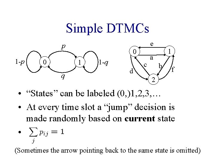
Simple DTMCs e p 1 -p 0 0 1 q 1 -q d c 1 a b f 2 • “States” can be labeled (0, )1, 2, 3, … • At every time slot a “jump” decision is made randomly based on current state • (Sometimes the arrow pointing back to the same state is omitted)

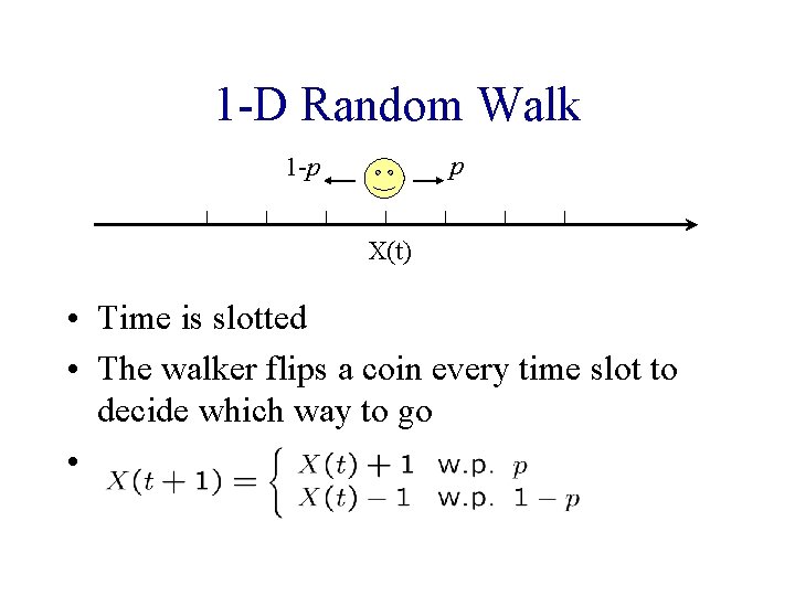
1 -D Random Walk p 1 -p X(t) • Time is slotted • The walker flips a coin every time slot to decide which way to go •

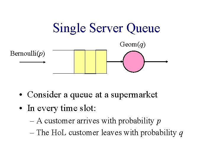
Single Server Queue Geom(q) Bernoulli(p) • Consider a queue at a supermarket • In every time slot: – A customer arrives with probability p – The Ho. L customer leaves with probability q

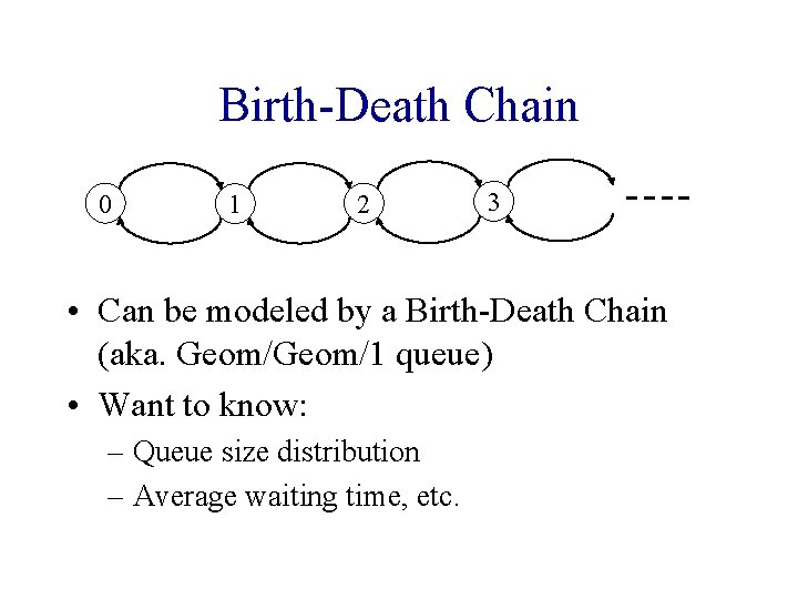
Birth-Death Chain 0 1 2 3 • Can be modeled by a Birth-Death Chain (aka. Geom/1 queue) • Want to know: – Queue size distribution – Average waiting time, etc.

Markov Property • “Future” is independent of “Past” given “Present” • In other words: Memoryless • We’ve seen memoryless distributions: Exponential and Geometric • Useful for modeling and analyzing real systems

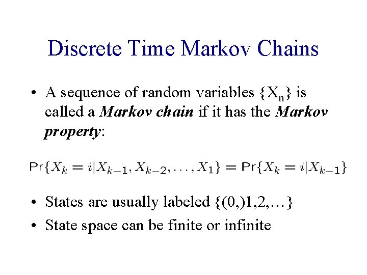
Discrete Time Markov Chains • A sequence of random variables {Xn} is called a Markov chain if it has the Markov property: • States are usually labeled {(0, )1, 2, …} • State space can be finite or infinite

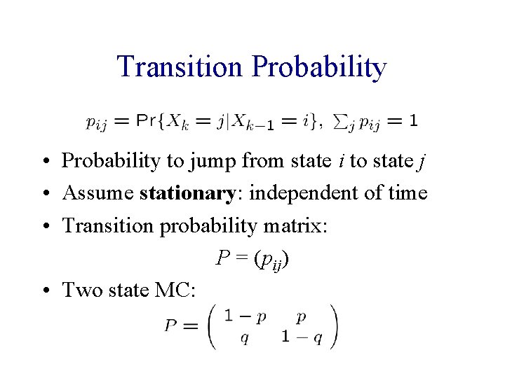
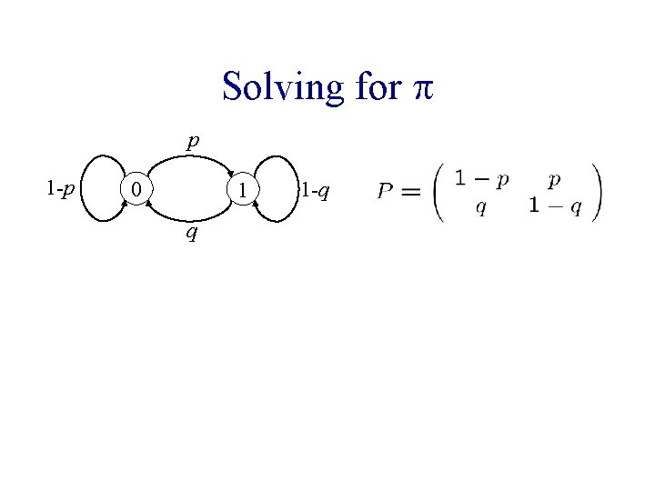
Transition Probability • Probability to jump from state i to state j • Assume stationary: independent of time • Transition probability matrix: P = (pij) • Two state MC:

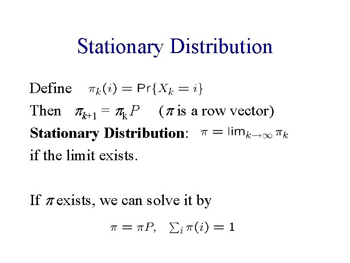
Stationary Distribution Define Then pk+1 = pk P (p is a row vector) Stationary Distribution: if the limit exists. If p exists, we can solve it by

Balance Equations • These are called balance equations – Transitions in and out of state i are balanced

In General • If we partition all the states into two sets, then transitions between the two sets must be “balanced”. – Equivalent to a bi-section in the state transition graph – This can be easily derived from the Balance Equations

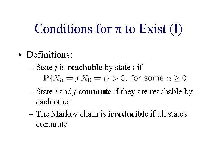
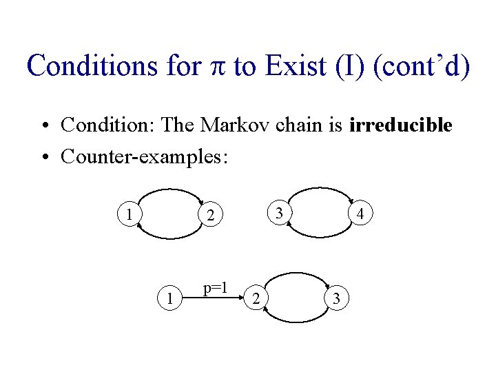
Conditions for p to Exist (I) • Definitions: – State j is reachable by state i if – State i and j commute if they are reachable by each other – The Markov chain is irreducible if all states commute

Conditions for p to Exist (I) (cont’d) • Condition: The Markov chain is irreducible • Counter-examples: 1 3 2 1 p=1 2 4 3

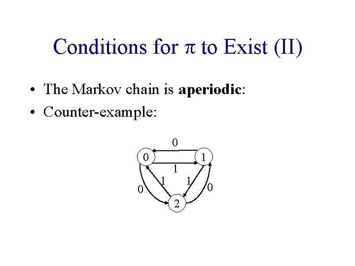
Conditions for p to Exist (II) • The Markov chain is aperiodic: • Counter-example: 0 0 0 1 1 2 1 1 0

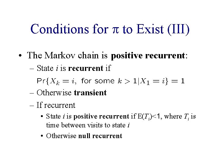
Conditions for p to Exist (III) • The Markov chain is positive recurrent: – State i is recurrent if – Otherwise transient – If recurrent • State i is positive recurrent if E(Ti)<1, where Ti is time between visits to state i • Otherwise null recurrent

Solving for p p 1 -p 0 1 q 1 -q

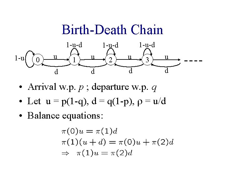
Birth-Death Chain 1 -u-d 1 -u 0 u d 1 1 -u-d u d 2 u d 3 u d • Arrival w. p. p ; departure w. p. q • Let u = p(1 -q), d = q(1 -p), r = u/d • Balance equations:

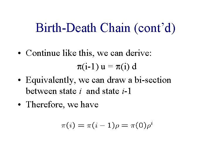
Birth-Death Chain (cont’d) • Continue like this, we can derive: p(i-1) u = p(i) d • Equivalently, we can draw a bi-section between state i and state i-1 • Therefore, we have

Birth-Death Chain (cont’d)

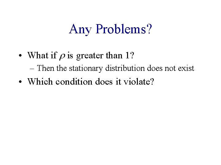
Any Problems? • What if r is greater than 1? – Then the stationary distribution does not exist • Which condition does it violate?

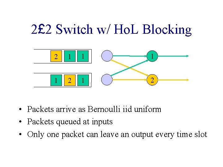
2£ 2 Switch w/ Ho. L Blocking 2 1 1 2 1 2 • Packets arrive as Bernoulli iid uniform • Packets queued at inputs • Only one packet can leave an output every time slot

2£ 2 Switch (cont’d) • If both Ho. L packets are destined to the same output – Only one of them is served (chosen randomly) – The other output is idle, as packets are blocked – This is called head of line blocking – Ho. L blocking reduces throughput • Want to know: throughput of this switch

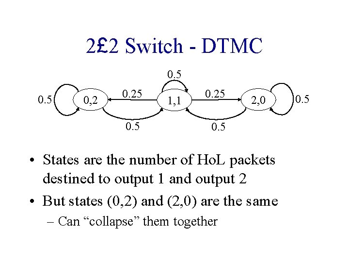
2£ 2 Switch - DTMC 0. 5 0, 2 0. 25 0. 5 1, 1 0. 25 2, 0 0. 5 • States are the number of Ho. L packets destined to output 1 and output 2 • But states (0, 2) and (2, 0) are the same – Can “collapse” them together 0. 5

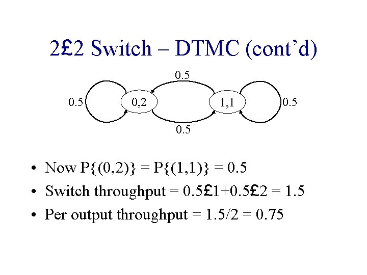
2£ 2 Switch – DTMC (cont’d) 0. 5 0, 2 1, 1 0. 5 • Now P{(0, 2)} = P{(1, 1)} = 0. 5 • Switch throughput = 0. 5£ 1+0. 5£ 2 = 1. 5 • Per output throughput = 1. 5/2 = 0. 75

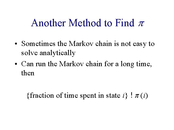
Another Method to Find p • Sometimes the Markov chain is not easy to solve analytically • Can run the Markov chain for a long time, then {fraction of time spent in state i} ! p (i)