Markov Decision Processes A Survey Martin L Puterman

Markov Decision Processes: A Survey Martin L. Puterman

Outline • • Example - Airline Meal Planning MDP Overview and Applications Airline Meal Planning Models and Results MDP Theory and Computation Bayesian MDPs and Censored Models Reinforcement Learning Concluding Remarks Martin L. Puterman - June 2002 2

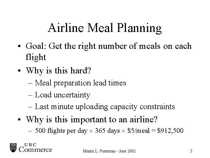
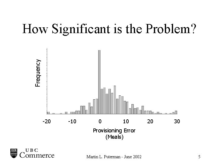
Airline Meal Planning • Goal: Get the right number of meals on each flight • Why is this hard? – Meal preparation lead times – Load uncertainty – Last minute uploading capacity constraints • Why is this important to an airline? – 500 flights per day 365 days $5/meal = $912, 500 Martin L. Puterman - June 2002 3

Martin L. Puterman - June 2002 4

Frequency How Significant is the Problem? -20 -10 0 10 20 30 Provisioning Error (Meals) Martin L. Puterman - June 2002 5

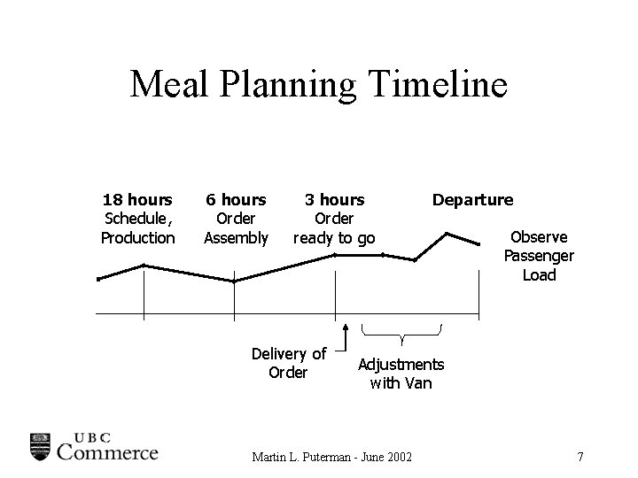
The Meal Planning Decision Process • At several key decision points up to 3 hours before departure, the meal planner observes reservations and meals allocated and adjusts allocated meal quantity. • Hourly in the last three hours, adjustments are made but the cost of adjustment is significantly higher and limited by delivery van capacity and uploading logistics. Martin L. Puterman - June 2002 6

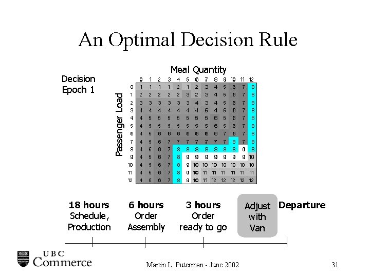
Meal Planning Timeline 18 hours Schedule, Production 6 hours Order Assembly 3 hours Order ready to go Delivery of Order Departure Observe Passenger Load Adjustments with Van Martin L. Puterman - June 2002 7

Airline Meal Planning Operational goal; develop a meal planning strategy that minimizes expected total overage, underage and operational costs A Meal Planning Strategy specifies at each decision point the number of extra meals to prepare or deliver for any observed meal allocation and reservation quantity. Martin L. Puterman - June 2002 8

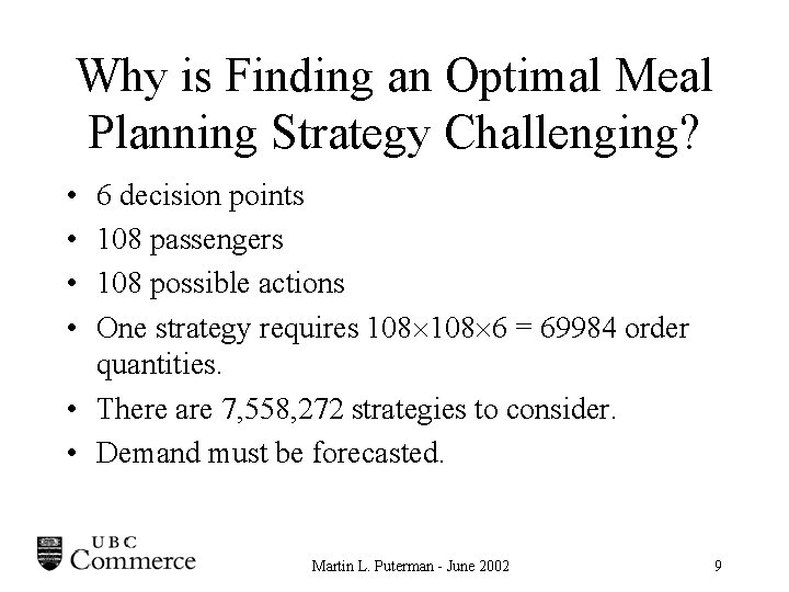
Why is Finding an Optimal Meal Planning Strategy Challenging? • • 6 decision points 108 passengers 108 possible actions One strategy requires 108 6 = 69984 order quantities. • There are 7, 558, 272 strategies to consider. • Demand must be forecasted. Martin L. Puterman - June 2002 9

Airline Meal Planning Characteristics • A similar decision is made at several time points • There are costs associated with each decision • The decision has future consequences • The overall cost depends on several events • There is uncertainty about the future Martin L. Puterman - June 2002 10

What is a Markov decision process? • A mathematical representation of a sequential decision making problem in which: – A system evolves through time. – A decision maker controls it by taking actions at pre-specified points of time. – Actions incur immediate costs or accrue immediate rewards and affect the subsequent system state. Martin L. Puterman - June 2002 11

MDP Overview Martin L. Puterman - June 2002 12

Markov Decision Processes are also known as: • • • MDPs Dynamic Programs Stochastic Dynamic Programs Sequential Decision Processes Stochastic Control Problems Martin L. Puterman - June 2002 13

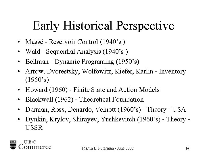
Early Historical Perspective • • Massé - Reservoir Control (1940’s ) Wald - Sequential Analysis (1940’s ) Bellman - Dynamic Programing (1950’s) Arrow, Dvorestsky, Wolfowitz, Kiefer, Karlin - Inventory (1950’s) Howard (1960) - Finite State and Action Models Blackwell (1962) - Theoretical Foundation Derman, Ross, Denardo, Veinott (1960’s) - Theory - USA Dynkin, Krylov, Shirayev, Yushkevitch (1960’s) - Theory USSR Martin L. Puterman - June 2002 14

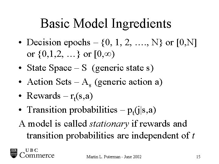
Basic Model Ingredients • Decision epochs – {0, 1, 2, …. , N} or [0, N] or {0, 1, 2, …} or [0, ) • State Space – S (generic state s) • Action Sets – As (generic action a) • Rewards – rt(s, a) • Transition probabilities – pt(j|s, a) A model is called stationary if rewards and transition probabilities are independent of t Martin L. Puterman - June 2002 15

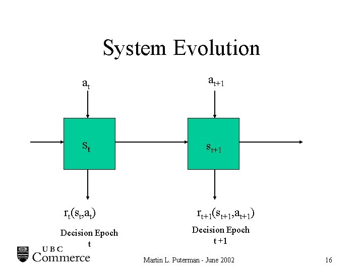
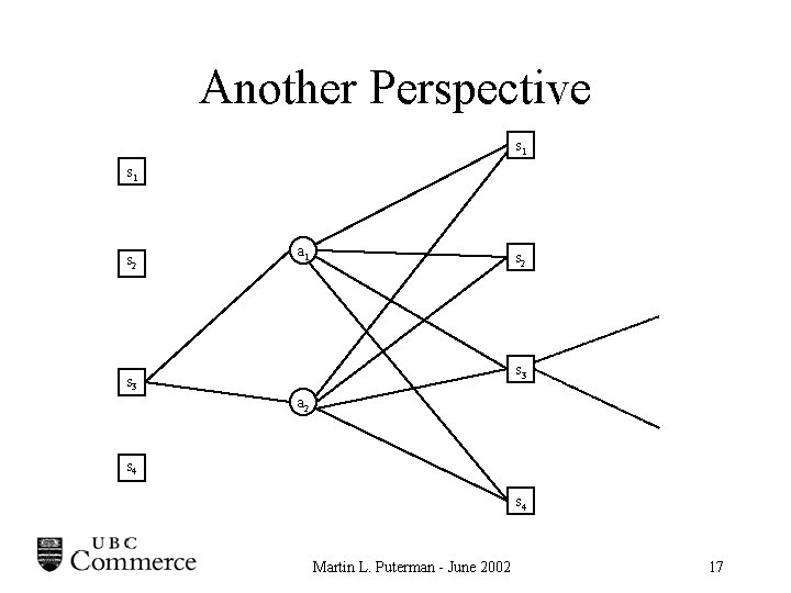
System Evolution at at+1 st st+1 rt(st, at) Decision Epoch t rt+1(st+1, at+1) Decision Epoch t +1 Martin L. Puterman - June 2002 16

Another Perspective s 1 s 2 a 1 s 2 s 3 a 2 s 4 Martin L. Puterman - June 2002 17

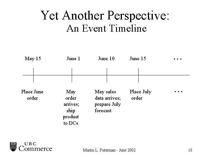
Yet Another Perspective: An Event Timeline May 15 Place June order June 1 May order arrives; ship product to DCs June 10 May sales data arrives; prepare July forecast June 15 Place July order Martin L. Puterman - June 2002 . . . 18

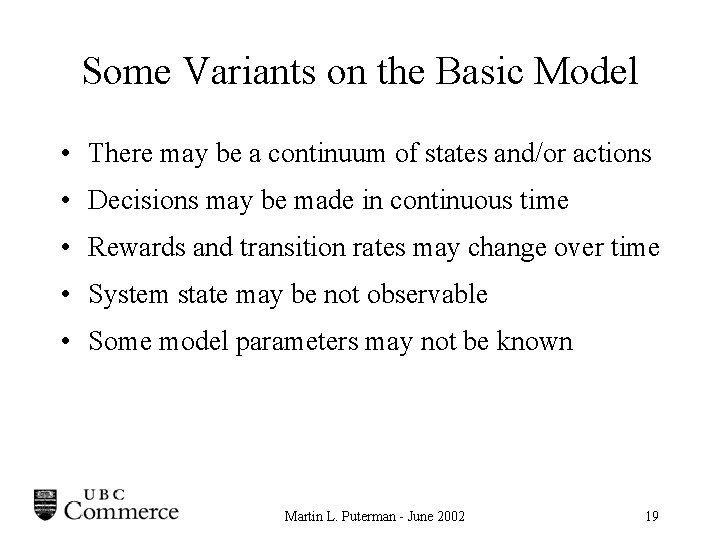
Some Variants on the Basic Model • There may be a continuum of states and/or actions • Decisions may be made in continuous time • Rewards and transition rates may change over time • System state may be not observable • Some model parameters may not be known Martin L. Puterman - June 2002 19

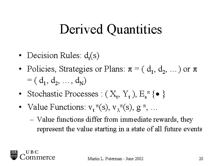
Derived Quantities • Decision Rules: dt(s) • Policies, Strategies or Plans: = ( d 1, d 2, …) or = ( d 1, d 2, …, d. N) • Stochastic Processes : ( Xt, Yt ), Es { } • Value Functions: vt (s), v (s), g , … – Value functions differ from immediate rewards, they represent the value starting in a state of all future events Martin L. Puterman - June 2002 20

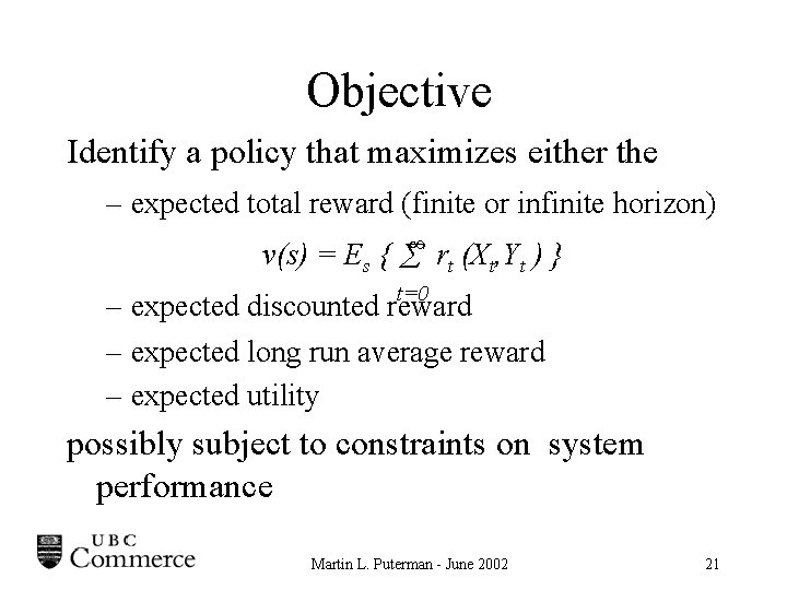
Objective Identify a policy that maximizes either the – expected total reward (finite or infinite horizon) v(s) = Es { rt (Xt, Yt ) } t=0 – expected discounted reward – expected long run average reward – expected utility possibly subject to constraints on system performance Martin L. Puterman - June 2002 21

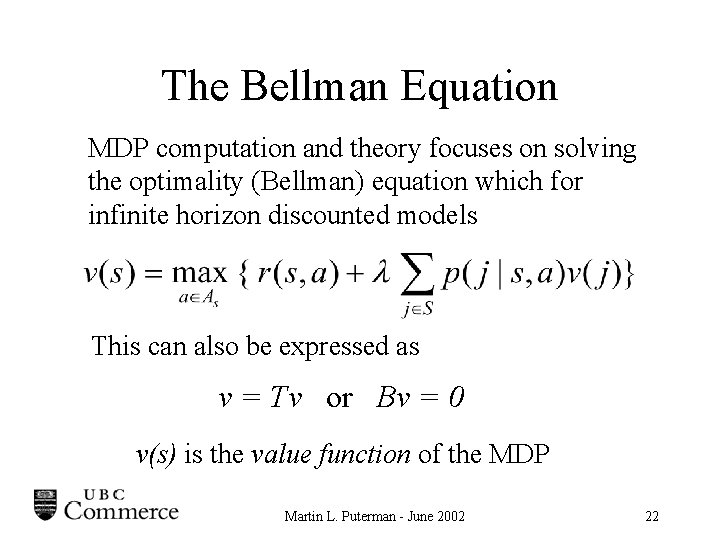
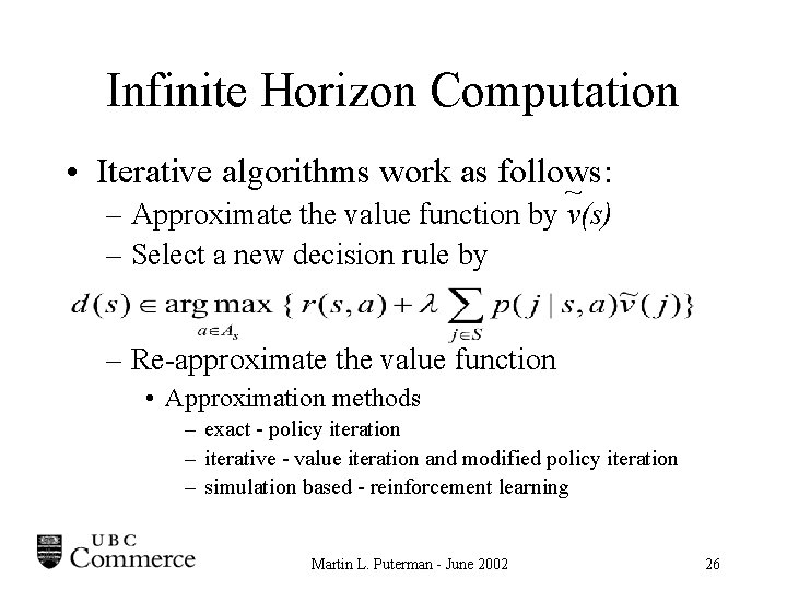
The Bellman Equation MDP computation and theory focuses on solving the optimality (Bellman) equation which for infinite horizon discounted models This can also be expressed as v = Tv or Bv = 0 v(s) is the value function of the MDP Martin L. Puterman - June 2002 22

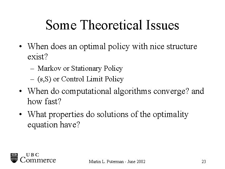
Some Theoretical Issues • When does an optimal policy with nice structure exist? – Markov or Stationary Policy – (s, S) or Control Limit Policy • When do computational algorithms converge? and how fast? • What properties do solutions of the optimality equation have? Martin L. Puterman - June 2002 23

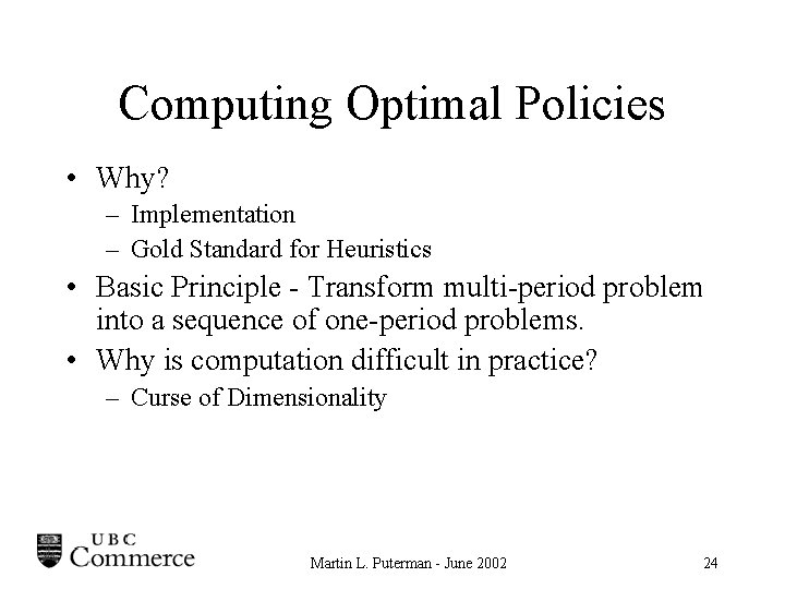
Computing Optimal Policies • Why? – Implementation – Gold Standard for Heuristics • Basic Principle - Transform multi-period problem into a sequence of one-period problems. • Why is computation difficult in practice? – Curse of Dimensionality Martin L. Puterman - June 2002 24

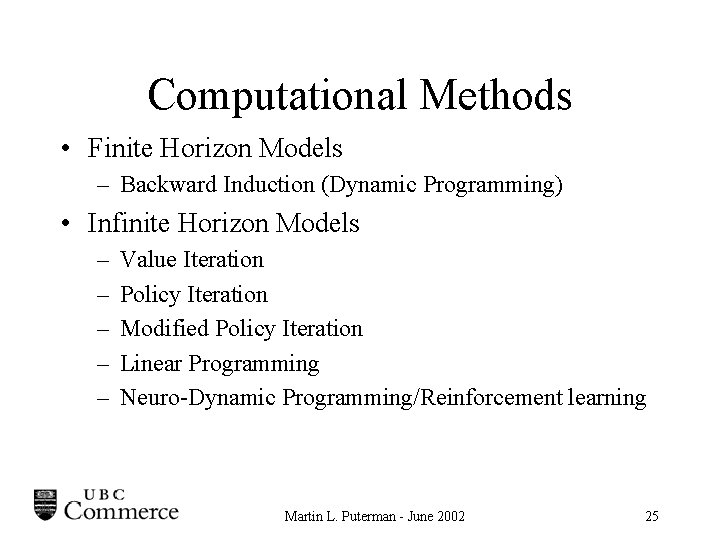
Computational Methods • Finite Horizon Models – Backward Induction (Dynamic Programming) • Infinite Horizon Models – – – Value Iteration Policy Iteration Modified Policy Iteration Linear Programming Neuro-Dynamic Programming/Reinforcement learning Martin L. Puterman - June 2002 25

Infinite Horizon Computation • Iterative algorithms work as follows: ~ – Approximate the value function by v(s) – Select a new decision rule by – Re-approximate the value function • Approximation methods – exact - policy iteration – iterative - value iteration and modified policy iteration – simulation based - reinforcement learning Martin L. Puterman - June 2002 26

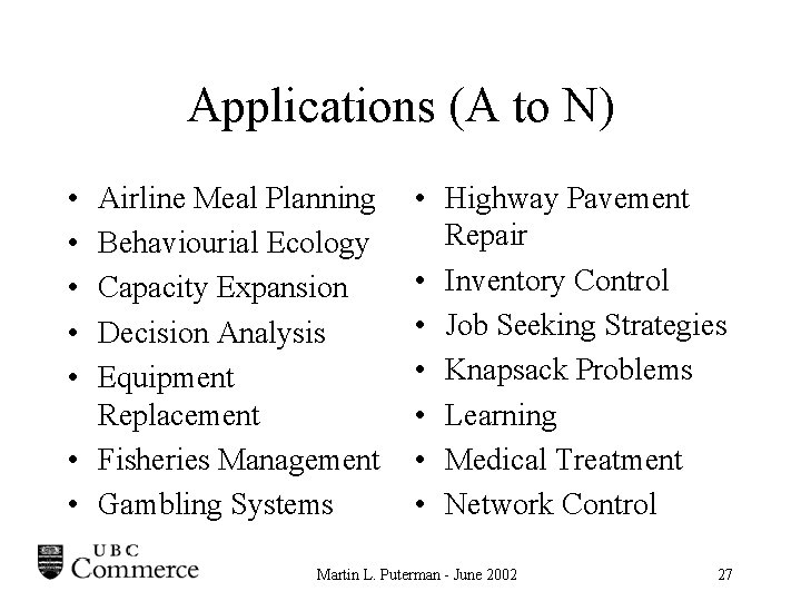
Applications (A to N) • • • Airline Meal Planning Behaviourial Ecology Capacity Expansion Decision Analysis Equipment Replacement • Fisheries Management • Gambling Systems • Highway Pavement Repair • Inventory Control • Job Seeking Strategies • Knapsack Problems • Learning • Medical Treatment • Network Control Martin L. Puterman - June 2002 27

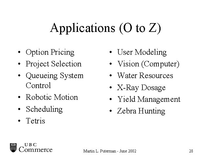
Applications (O to Z) • Option Pricing • Project Selection • Queueing System Control • Robotic Motion • Scheduling • Tetris • • • User Modeling Vision (Computer) Water Resources X-Ray Dosage Yield Management Zebra Hunting Martin L. Puterman - June 2002 28

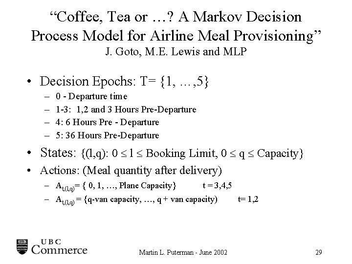
“Coffee, Tea or …? A Markov Decision Process Model for Airline Meal Provisioning” J. Goto, M. E. Lewis and MLP • Decision Epochs: T= {1, …, 5} – – 0 - Departure time 1 -3: 1, 2 and 3 Hours Pre-Departure 4: 6 Hours Pre - Departure 5: 36 Hours Pre-Departure • States: {(l, q): 0 l Booking Limit, 0 q Capacity} • Actions: (Meal quantity after delivery) – At, (l, q)= { 0, 1, …, Plane Capacity} t = 3, 4, 5 – At, (l, q) = {q-van capacity, …, q + van capacity) Martin L. Puterman - June 2002 t= 1, 2 29

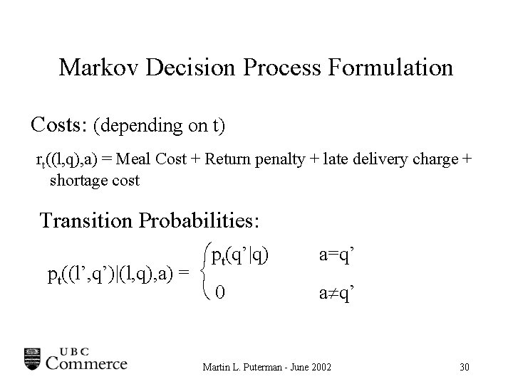
Markov Decision Process Formulation Costs: (depending on t) rt((l, q), a) = Meal Cost + Return penalty + late delivery charge + shortage cost Transition Probabilities: pt(q’|q) pt((l’, q’)|(l, q), a) = 0 a=q’ a q’ Martin L. Puterman - June 2002 30

An Optimal Decision Rule 18 hours Schedule, Production Passenger Load Decision Epoch 1 Meal Quantity 6 hours Order Assembly 3 hours Order ready to go Martin L. Puterman - June 2002 Adjust Departure with Van 31

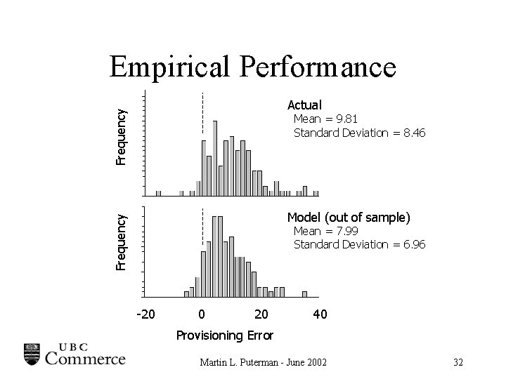
Empirical Performance Frequency Actual Mean = 9. 81 Standard Deviation = 8. 46 Frequency Model (out of sample) Mean = 7. 99 Standard Deviation = 6. 96 -20 0 20 40 Provisioning Error Martin L. Puterman - June 2002 32

Overage versus Shortage • Evaluate the model over a range of terminal costs • Observe the relationship of average overage and proportion of flights short-catered • 55 flight number / aircraft capacity combinations (evaluated separately) Martin L. Puterman - June 2002 33

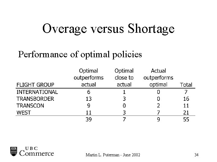
Overage versus Shortage Performance of optimal policies Martin L. Puterman - June 2002 34

Information Acquisition Martin L. Puterman - June 2002 35

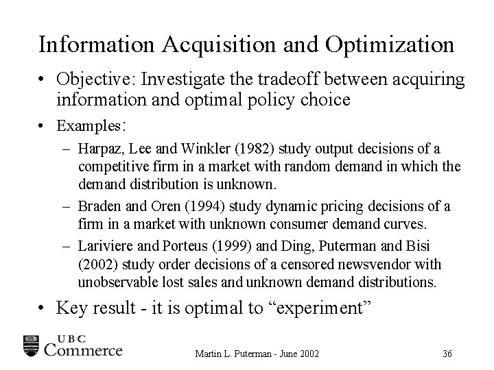
Information Acquisition and Optimization • Objective: Investigate the tradeoff between acquiring information and optimal policy choice • Examples: – Harpaz, Lee and Winkler (1982) study output decisions of a competitive firm in a market with random demand in which the demand distribution is unknown. – Braden and Oren (1994) study dynamic pricing decisions of a firm in a market with unknown consumer demand curves. – Lariviere and Porteus (1999) and Ding, Puterman and Bisi (2002) study order decisions of a censored newsvendor with unobservable lost sales and unknown demand distributions. • Key result - it is optimal to “experiment” Martin L. Puterman - June 2002 36

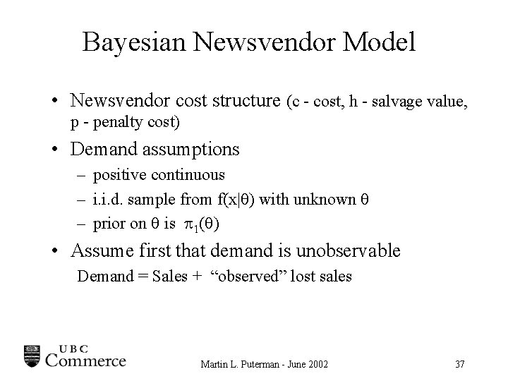
Bayesian Newsvendor Model • Newsvendor cost structure (c - cost, h - salvage value, p - penalty cost) • Demand assumptions – positive continuous – i. i. d. sample from f(x| ) with unknown – prior on is 1( ) • Assume first that demand is unobservable Demand = Sales + “observed” lost sales Martin L. Puterman - June 2002 37

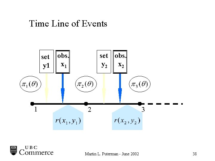
Time Line of Events set y 1 1 obs. x 1 set obs. y 2 x 2 2 Martin L. Puterman - June 2002 3 38

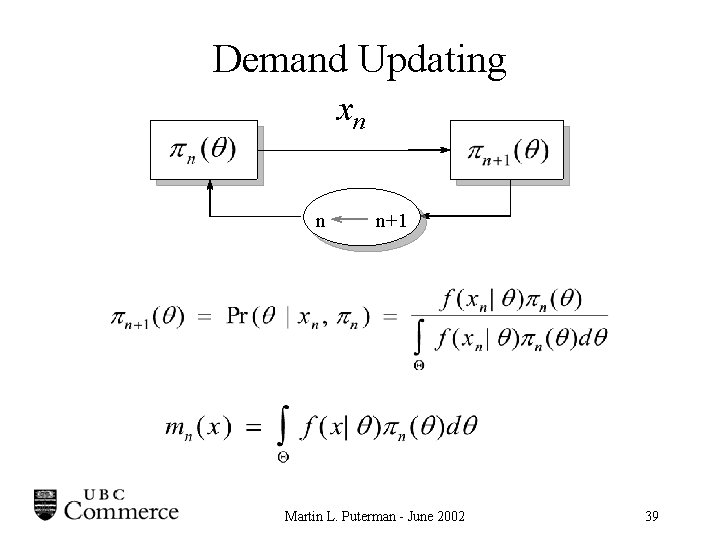
Demand Updating xn n n+1 Martin L. Puterman - June 2002 39

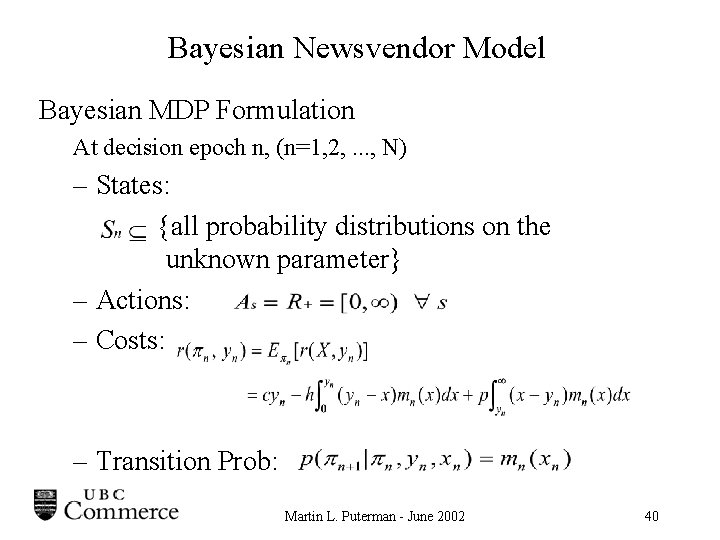
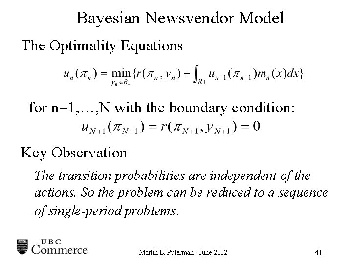
Bayesian Newsvendor Model Bayesian MDP Formulation At decision epoch n, (n=1, 2, . . . , N) – States: {all probability distributions on the unknown parameter} – Actions: – Costs: – Transition Prob: Martin L. Puterman - June 2002 40

Bayesian Newsvendor Model The Optimality Equations for n=1, …, N with the boundary condition: Key Observation The transition probabilities are independent of the actions. So the problem can be reduced to a sequence of single-period problems. Martin L. Puterman - June 2002 41

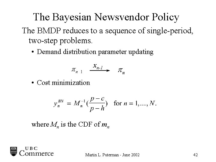
The Bayesian Newsvendor Policy The BMDP reduces to a sequence of single-period, two-step problems. • Demand distribution parameter updating xn-1 • Cost minimization where Mn is the CDF of mn Martin L. Puterman - June 2002 42

Bayesian Newsvendor with Unobservable Lost Sales • Model Set-up – Same as fully observable case but unmet demand is lost and unobservable • Question – Is the Bayesian Newsvendor policy optimal? Martin L. Puterman - June 2002 43

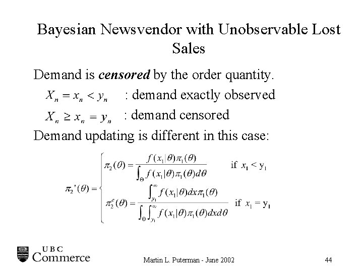
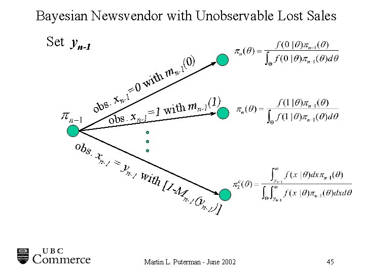
Bayesian Newsvendor with Unobservable Lost Sales Demand is censored by the order quantity. : demand exactly observed : demand censored Demand updating is different in this case: Martin L. Puterman - June 2002 44

Bayesian Newsvendor with Unobservable Lost Sales Set yn-1 0) ( -1 0 = -1 mn h t wi xn ) 1. ( s m 1 b n ith o w 1 = obs. x n-1 obs . x n-1 =y n-1 wit h [1 -M n-1 (y n -1 ) ] Martin L. Puterman - June 2002 45

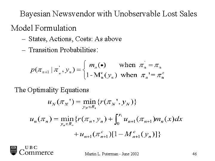
Bayesian Newsvendor with Unobservable Lost Sales Model Formulation – States, Actions, Costs: As above – Transition Probabilities: The Optimality Equations Martin L. Puterman - June 2002 46

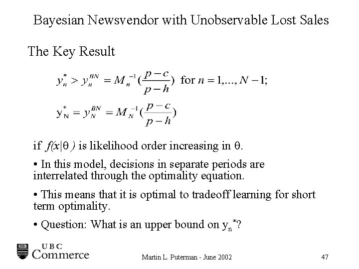
Bayesian Newsvendor with Unobservable Lost Sales The Key Result if f(x| ) is likelihood order increasing in . • In this model, decisions in separate periods are interrelated through the optimality equation. • This means that it is optimal to tradeoff learning for short term optimality. • Question: What is an upper bound on yn*? Martin L. Puterman - June 2002 47

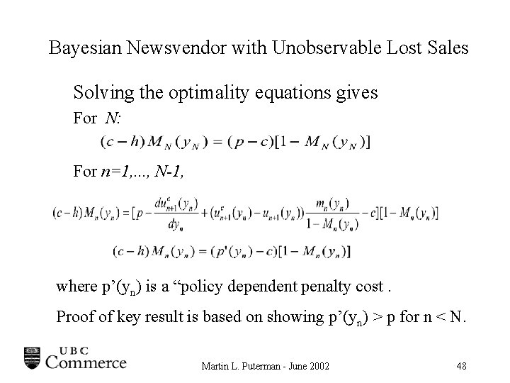
Bayesian Newsvendor with Unobservable Lost Sales Solving the optimality equations gives For N: For n=1, . . . , N-1, where p’(yn) is a “policy dependent penalty cost. Proof of key result is based on showing p’(yn) > p for n < N. Martin L. Puterman - June 2002 48

Bayesian Newsvendor with Unobservable Lost Sales • Some comments – The extra penalty can be interpreted as the marginal expected value of information at decision epoch n. – Numerical results show small improvements when using the optimal policy as opposed to the Bayesian Newsvendor policy. – We have extended this to a two level supply chain Martin L. Puterman - June 2002 49

Partially Observed MDPs • In POMDPs, system state is not observable. – Decision maker receives a signal y which is related to the system state by q(y|s, a). • Analysis is based on using Bayes Theorem to estimate distribution of the system state given the signal – Similar to Bayesian MDPs described above • the posterior state distribution is a sufficient statistic for decision making – State space is a continuum – Early work by Smallwood and Sondik (1972) • Applications – Medical diagnosis and treatment – Equipment repair Martin L. Puterman - June 2002 50

Reinforcement Learning and Neuro-Dynamic Programming Martin L. Puterman - June 2002 51

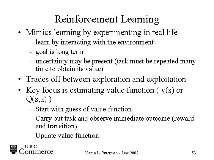
Neuro-Dynamic Programming or Reinforcement Learning • A different way to think about dynamic programming – Basis in artificial intelligence research – Mimics learning behavior of animals • Developed to: – Solve problems with high dimensional state spaces and/or – Solve problems in which the system is described by a simulator (as opposed to a mathematical model) • NDL/Rl refers to a collection of methods combining Monte Carlo methods with MDP concepts Martin L. Puterman - June 2002 52

Reinforcement Learning • Mimics learning by experimenting in real life – learn by interacting with the environment – goal is long term – uncertainty may be present (task must be repeated many time to obtain its value) • Trades off between exploration and exploitation • Key focus is estimating value function ( v(s) or Q(s, a) ) – Start with guess of value function – Carry out task and observe immediate outcome (reward and transition) – Update value function Martin L. Puterman - June 2002 53

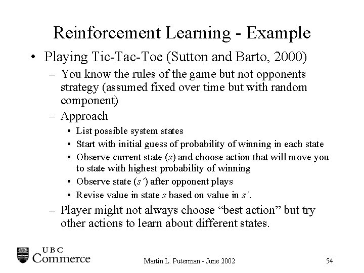
Reinforcement Learning - Example • Playing Tic-Tac-Toe (Sutton and Barto, 2000) – You know the rules of the game but not opponents strategy (assumed fixed over time but with random component) – Approach • List possible system states • Start with initial guess of probability of winning in each state • Observe current state (s) and choose action that will move you to state with highest probability of winning • Observe state (s’) after opponent plays • Revise value in state s based on value in s’. – Player might not always choose “best action” but try other actions to learn about different states. Martin L. Puterman - June 2002 54

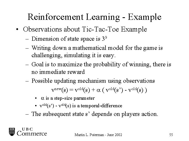
Reinforcement Learning - Example • Observations about Tic-Tac-Toe Example – Dimension of state space is 39 – Writing down a mathematical model for the game is challenging, simulating it is easy. – Goal is to maximize the probability of winning, there is no immediate reward – Possible updating mechanism using observations vnew(s) = vold(s) + ( vold(s’) - vold(s) ) • is a step-size parameter • vold(s’) - vold(s) is a temporal-difference – The subsequent state s’ depends on players action. Martin L. Puterman - June 2002 55

Reinforcement Learning Problems can be classified in two ways Martin L. Puterman - June 2002 56

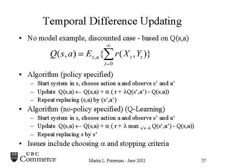
Temporal Difference Updating • No model example, discounted case - based on Q(s, a) • Algorithm (policy specified) – Start system in s, choose action a and observe s’ and a’ – Update Q(s, a) + ( r + Q(s’, a’) - Q(s, a)) – Repeat replacing (s, a) by (s’, a’) • Algorithm (no-policy specified) (Q-Learning) – Start system in s, choose action a and observe s’ and a’ – Update Q(s, a) + ( r + max a’ A Q(s’, a’) - Q(s, a)) – Repeat replacing s by s’ • Issues include choosing and stopping criteria Martin L. Puterman - June 2002 57

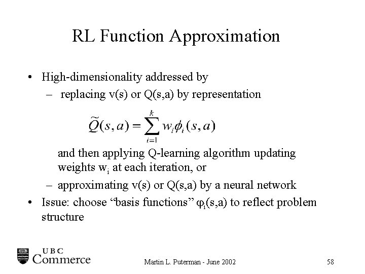
RL Function Approximation • High-dimensionality addressed by – replacing v(s) or Q(s, a) by representation and then applying Q-learning algorithm updating weights wi at each iteration, or – approximating v(s) or Q(s, a) by a neural network • Issue: choose “basis functions” i(s, a) to reflect problem structure Martin L. Puterman - June 2002 58

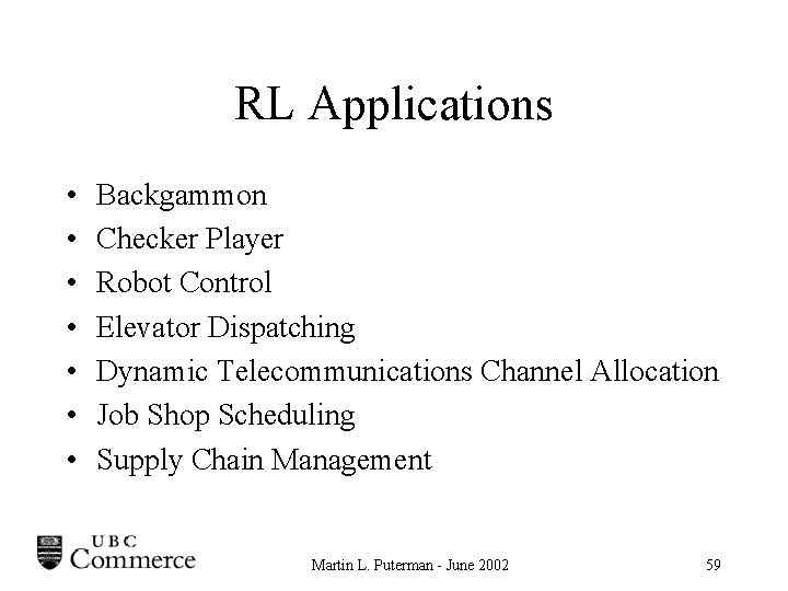
RL Applications • • Backgammon Checker Player Robot Control Elevator Dispatching Dynamic Telecommunications Channel Allocation Job Shop Scheduling Supply Chain Management Martin L. Puterman - June 2002 59

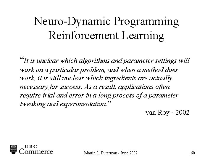
Neuro-Dynamic Programming Reinforcement Learning “It is unclear which algorithms and parameter settings will work on a particular problem, and when a method does work, it is still unclear which ingredients are actually necessary for success. As a result, applications often require trial and error in a long process of a parameter tweaking and experimentation. ” van Roy - 2002 Martin L. Puterman - June 2002 60

Conclusions Martin L. Puterman - June 2002 61

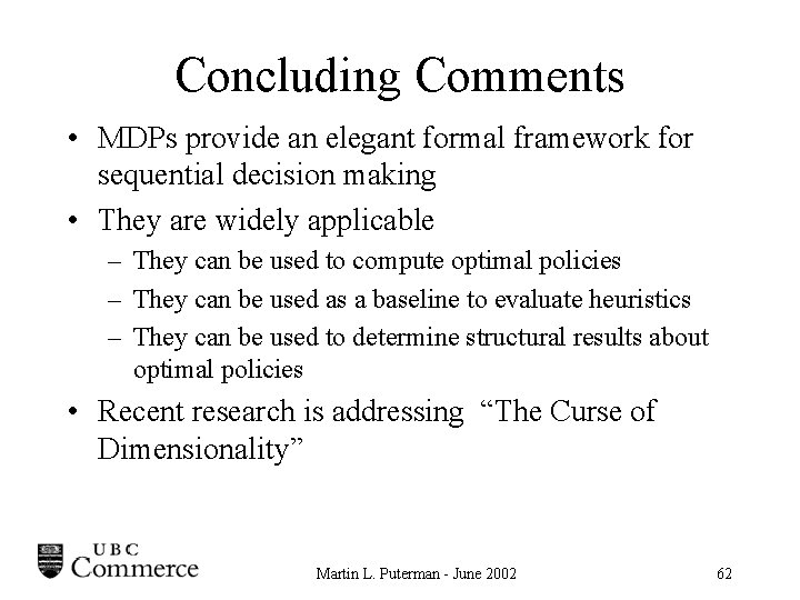
Concluding Comments • MDPs provide an elegant formal framework for sequential decision making • They are widely applicable – They can be used to compute optimal policies – They can be used as a baseline to evaluate heuristics – They can be used to determine structural results about optimal policies • Recent research is addressing “The Curse of Dimensionality” Martin L. Puterman - June 2002 62

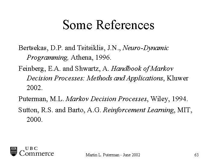
Some References Bertsekas, D. P. and Tsitsiklis, J. N. , Neuro-Dynamic Programming, Athena, 1996. Feinberg, E. A. and Shwartz, A. Handbook of Markov Decision Processes: Methods and Applications, Kluwer 2002. Puterman, M. L. Markov Decision Processes, Wiley, 1994. Sutton, R. S. and Barto, A. G. Reinforcement Learning, MIT, 2000. Martin L. Puterman - June 2002 63