Factor Graphs for Time Series Structured Optimization Class

Factor Graphs for Time Series Structured Optimization Class 23. 20 Nov 2014 Instructor: Gary Overett 20 Nov 2014 11755/18979 1

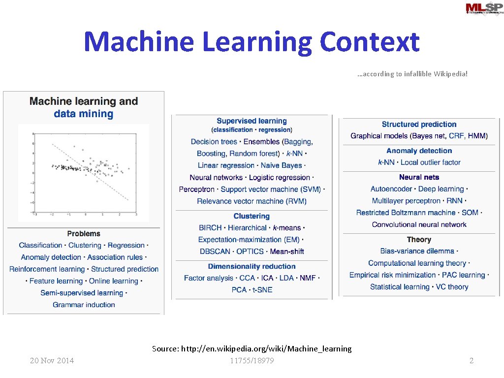
Machine Learning Context …according to infallible Wikipedia! Source: http: //en. wikipedia. org/wiki/Machine_learning 20 Nov 2014 11755/18979 2

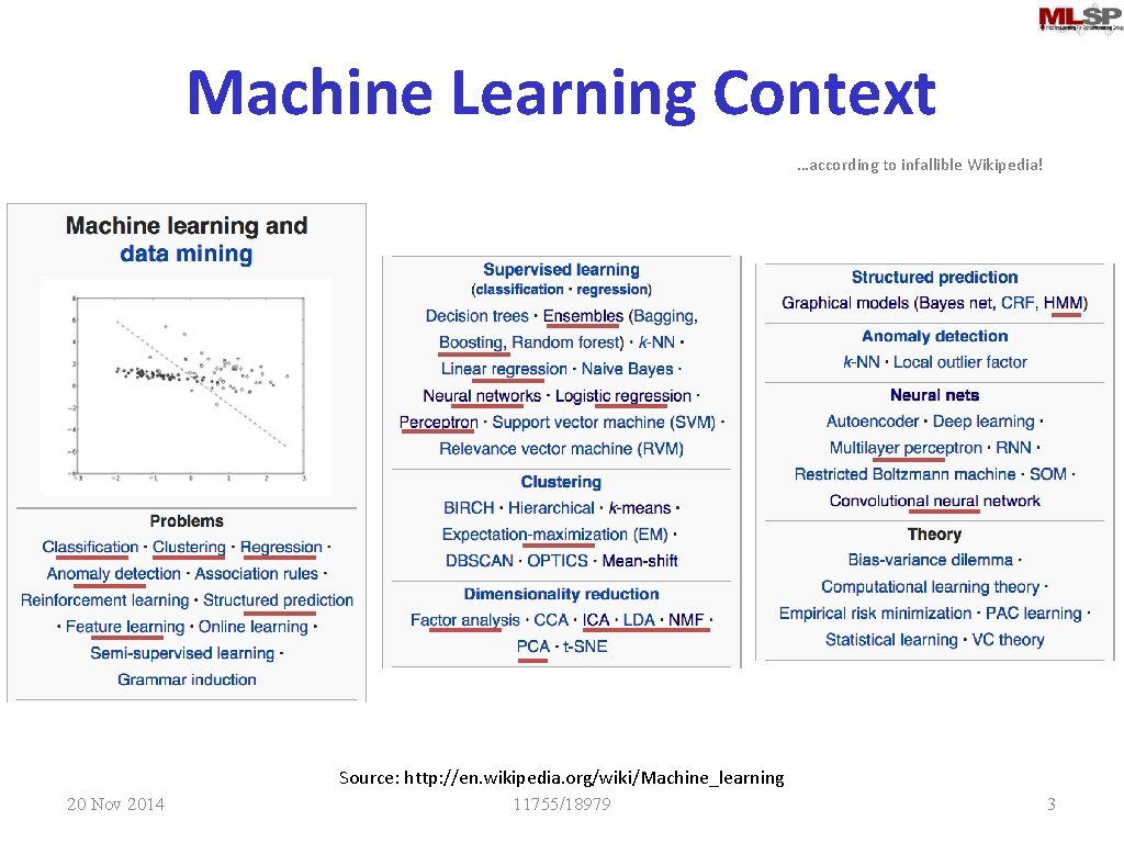
Machine Learning Context …according to infallible Wikipedia! Source: http: //en. wikipedia. org/wiki/Machine_learning 20 Nov 2014 11755/18979 3

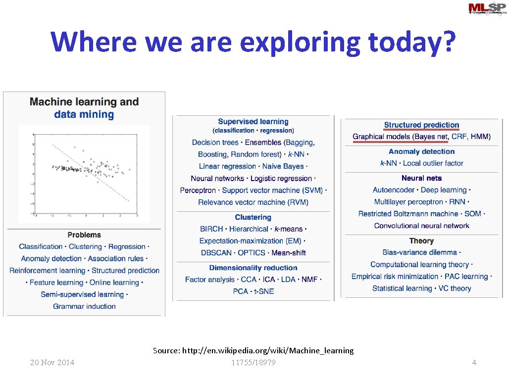
Where we are exploring today? Source: http: //en. wikipedia. org/wiki/Machine_learning 20 Nov 2014 11755/18979 4

What might you know about your “signal(s)”? • • • Gaussian Distribution Made up of Independent Components Face-like Clustered Sparse Locally Smooth (or should be!) 20 Nov 2014 11755/18979 5

What might you know about your “signal(s)”? • • Gaussian Distribution Made up of Independent Components Face-like Clustered Sparse Locally Smooth (or should be!) Choose or derive your constraints! 20 Nov 2014 11755/18979 6

The more I know about my signal (or the signal I am trying to estimate) the more constraints I’m able to reasonably apply! 20 Nov 2014 11755/18979 7

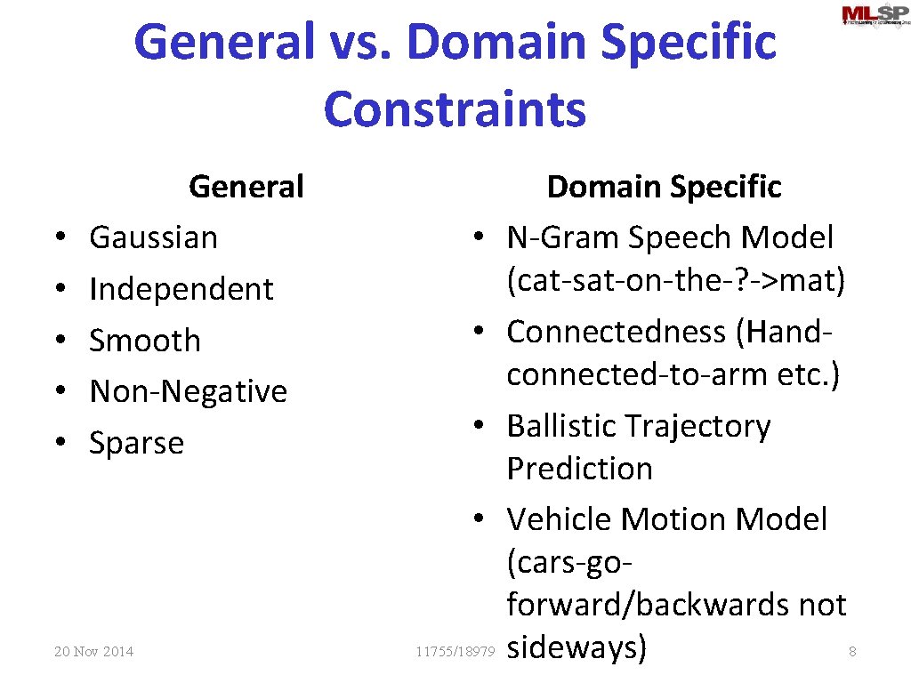
General vs. Domain Specific Constraints • • • General Gaussian Independent Smooth Non-Negative Sparse • • 20 Nov 2014 11755/18979 Domain Specific N-Gram Speech Model (cat-sat-on-the-? ->mat) Connectedness (Handconnected-to-arm etc. ) Ballistic Trajectory Prediction Vehicle Motion Model (cars-goforward/backwards not 8 sideways)

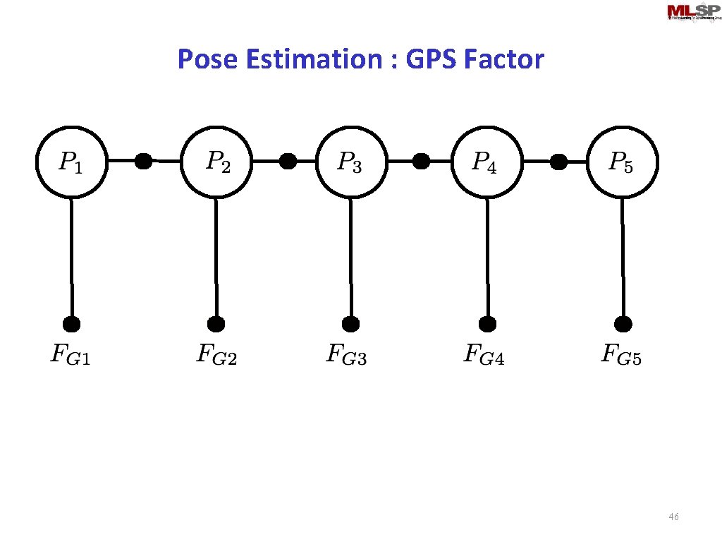
Consider the following ‘signal’ We want to know the position of a survey vehicle in the real world. Given the following time-series information: • • GPS location data at 1 Hz (may suffer dropout) Wheel Encoder Odometry Measurements every 2 m Inertial Sensor Measurements (Gyroscope) every 2 m Basic Vehicle Geometry (wheel base width etc. ) 20 Nov 2014 11755/18979 9

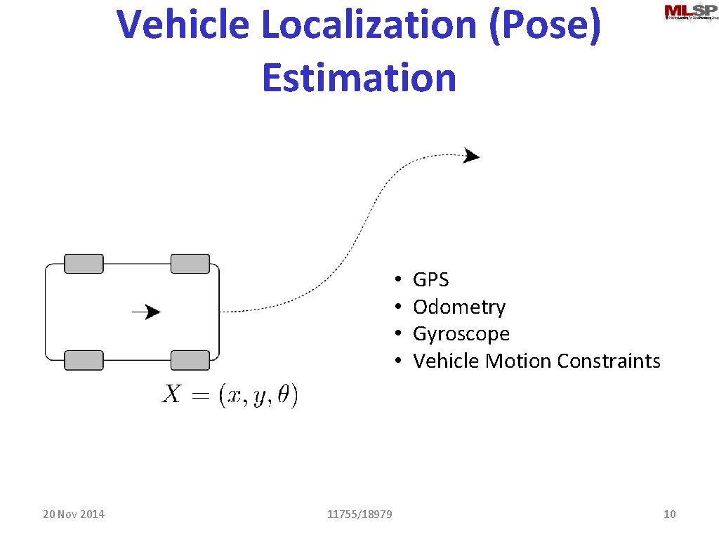
Vehicle Localization (Pose) Estimation • • 20 Nov 2014 11755/18979 GPS Odometry Gyroscope Vehicle Motion Constraints 10

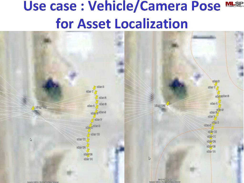
Use case : Vehicle/Camera Pose for Asset Localization 20 Nov 2014 11755/18979 11

Kalman Filter : Fail! 20 Nov 2014 11755/18979 12

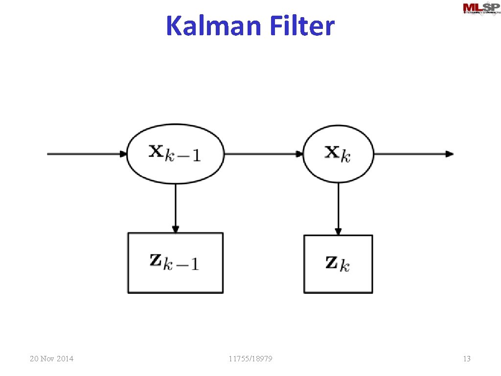
Kalman Filter 20 Nov 2014 11755/18979 13

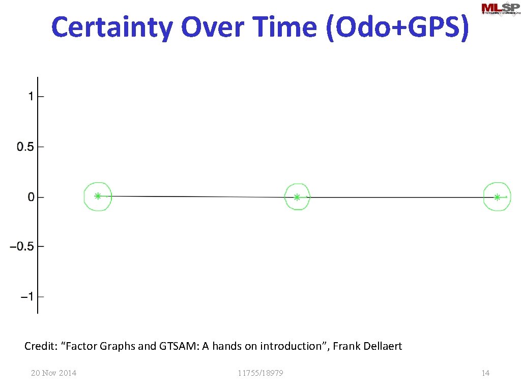
Certainty Over Time (Odo+GPS) Credit: “Factor Graphs and GTSAM: A hands on introduction”, Frank Dellaert 20 Nov 2014 11755/18979 14

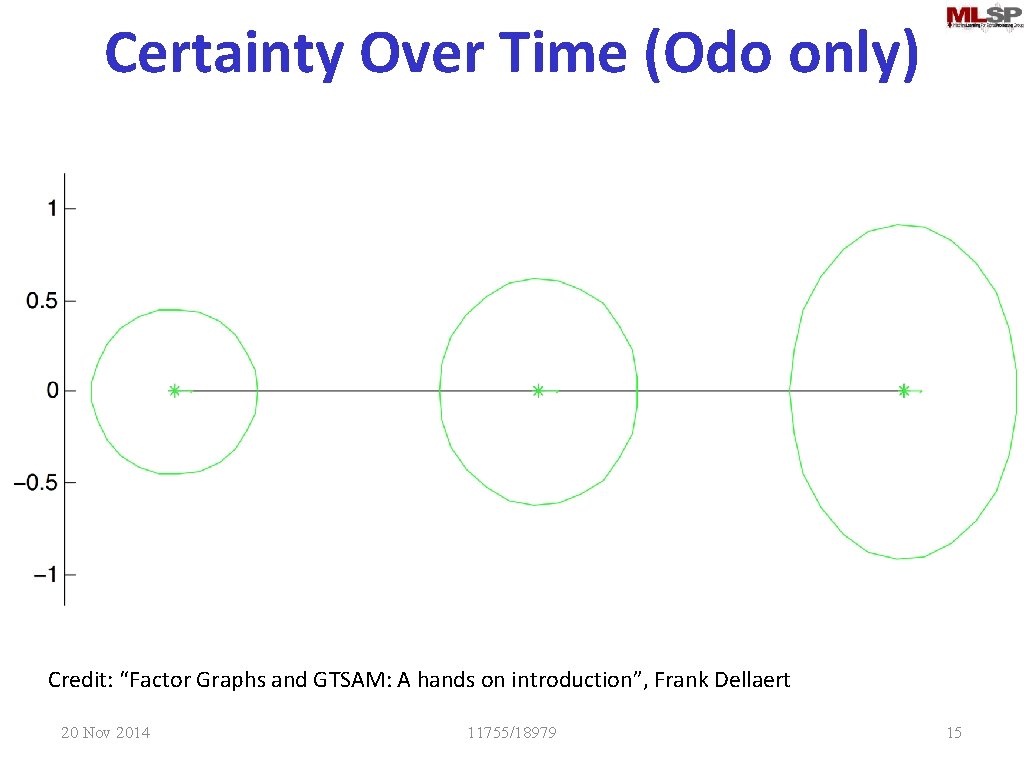
Certainty Over Time (Odo only) Credit: “Factor Graphs and GTSAM: A hands on introduction”, Frank Dellaert 20 Nov 2014 11755/18979 15

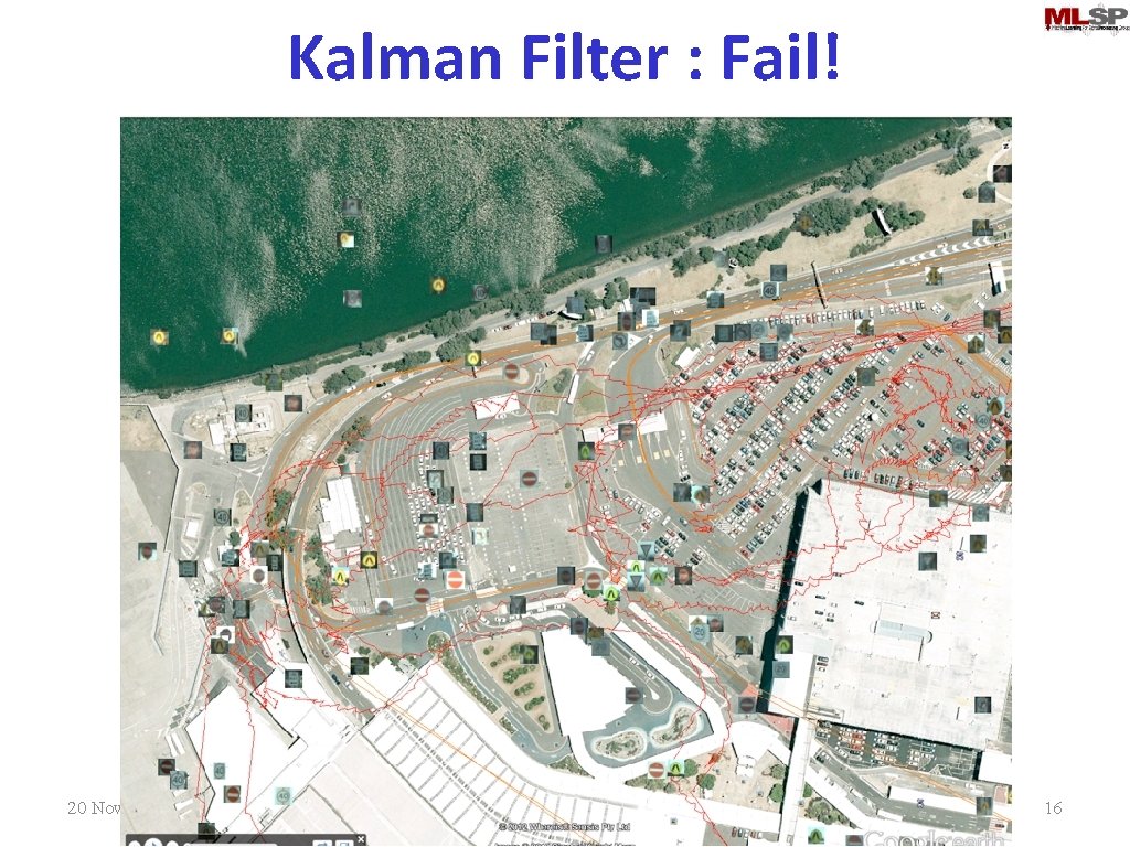
Kalman Filter : Fail! 20 Nov 2014 11755/18979 16

Survey Vehicle : Signal Behavior • GPS Suffers Dropout, Noise and Discontinuities • Odometry is very robust but multiple paths can explain a given odometry • Gyroscope is has a high precision but ‘drifts’ • Vehicles travel along relatively smooth paths. Normal operation excludes lateral (sideways) motion. • These constraints suggest a structured (graphical) prediction approach. 20 Nov 2014 11755/18979 17

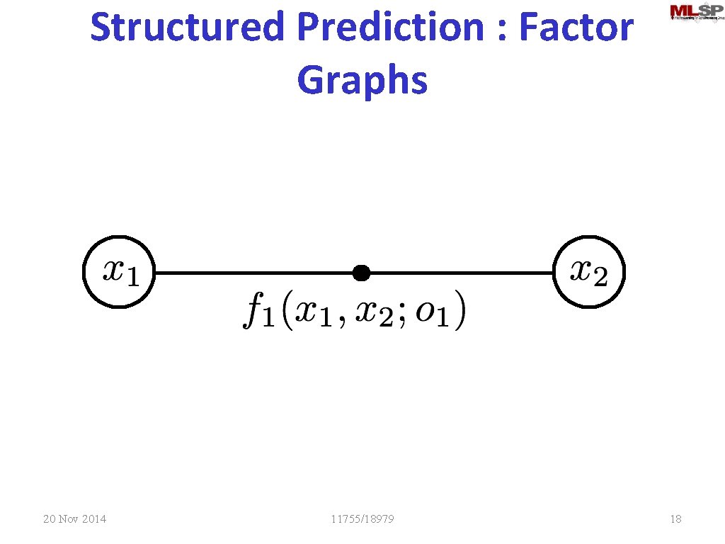
Structured Prediction : Factor Graphs 20 Nov 2014 11755/18979 18

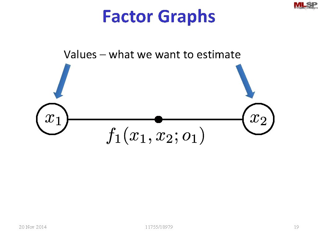
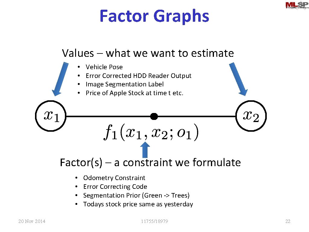
Factor Graphs Values – what we want to estimate 20 Nov 2014 11755/18979 19

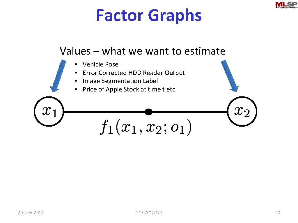
Factor Graphs Values – what we want to estimate • • 20 Nov 2014 Vehicle Pose Error Corrected HDD Reader Output Image Segmentation Label Price of Apple Stock at time t etc. 11755/18979 20

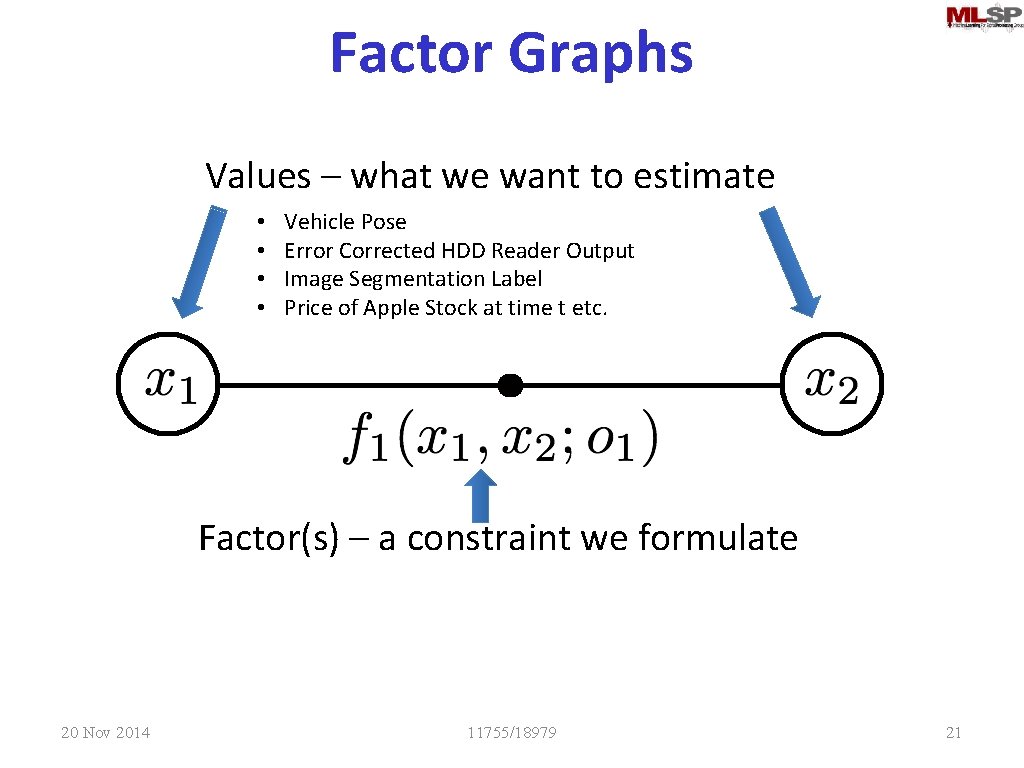
Factor Graphs Values – what we want to estimate • • Vehicle Pose Error Corrected HDD Reader Output Image Segmentation Label Price of Apple Stock at time t etc. Factor(s) – a constraint we formulate 20 Nov 2014 11755/18979 21

Factor Graphs Values – what we want to estimate • • Vehicle Pose Error Corrected HDD Reader Output Image Segmentation Label Price of Apple Stock at time t etc. Factor(s) – a constraint we formulate • • 20 Nov 2014 Odometry Constraint Error Correcting Code Segmentation Prior (Green -> Trees) Todays stock price same as yesterday 11755/18979 22

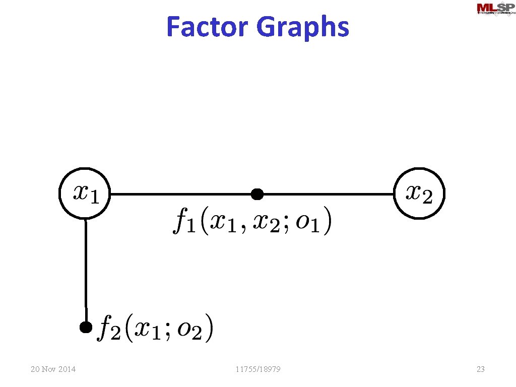
Factor Graphs 20 Nov 2014 11755/18979 23

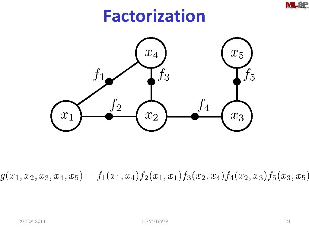
Factorization 20 Nov 2014 11755/18979 24

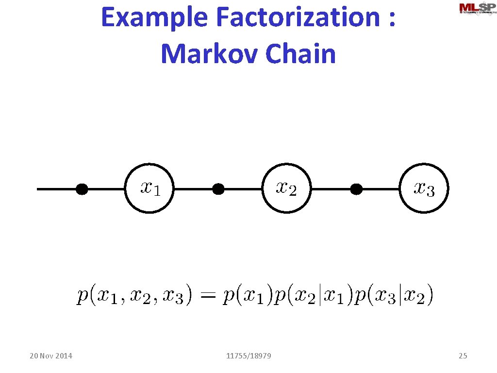
Example Factorization : Markov Chain 20 Nov 2014 11755/18979 25

Unifying View of… • • • Markov random fields Kalman Filters HMM’s Parity Codes Bayesian Networks 20 Nov 2014 11755/18979 26

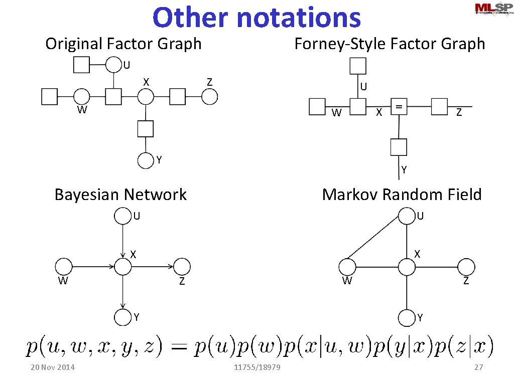
Other notations Forney-Style Factor Graph Original Factor Graph U Z X U W Y Y Bayesian Network Markov Random Field U U X X W W Z Y 20 Nov 2014 Z X W Z Y 11755/18979 27

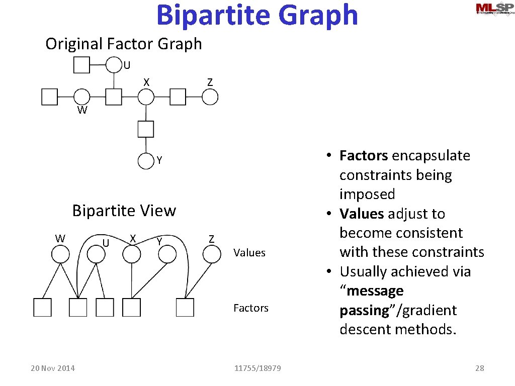
Bipartite Graph Original Factor Graph U Z X W Y Bipartite View W U X Y Z Values Factors 20 Nov 2014 11755/18979 • Factors encapsulate constraints being imposed • Values adjust to become consistent with these constraints • Usually achieved via “message passing”/gradient descent methods. 28

Optimization • • • Several algorithms are used Random vs “Best Guess” initialization Gauss-Newton Stepping Levenberg-Marquart Message Passing Algorithms Structure dependent/exploiting optimization strategies – ISAM 2 (for SLAM problems) 20 Nov 2014 11755/18979 29

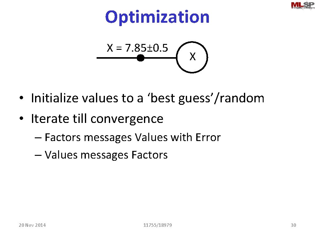
Optimization X = 7. 85± 0. 5 X • Initialize values to a ‘best guess’/random • Iterate till convergence – Factors messages Values with Error – Values messages Factors 20 Nov 2014 11755/18979 30

Optimization X = 7. 85± 0. 5 X=0 • Initialize values to a ‘best guess’/random • Iterate till convergence – Factors messages Values with Error – Values messages Factors 20 Nov 2014 11755/18979 31

Optimization X = 7. 85± 0. 5 X=5 • Initialize values to a ‘best guess’/random • Iterate till convergence – Factors messages Values with Error – Values messages Factors 20 Nov 2014 11755/18979 32

Optimization X = 7. 85± 0. 5 X=7 • Initialize values to a ‘best guess’/random • Iterate till convergence – Factors messages Values with Error – Values messages Factors 20 Nov 2014 11755/18979 33

Optimization X = 7. 85± 0. 5 X=7. 5 • Initialize values to a ‘best guess’/random • Iterate till convergence – Factors messages Values with Error – Values messages Factors 20 Nov 2014 11755/18979 34

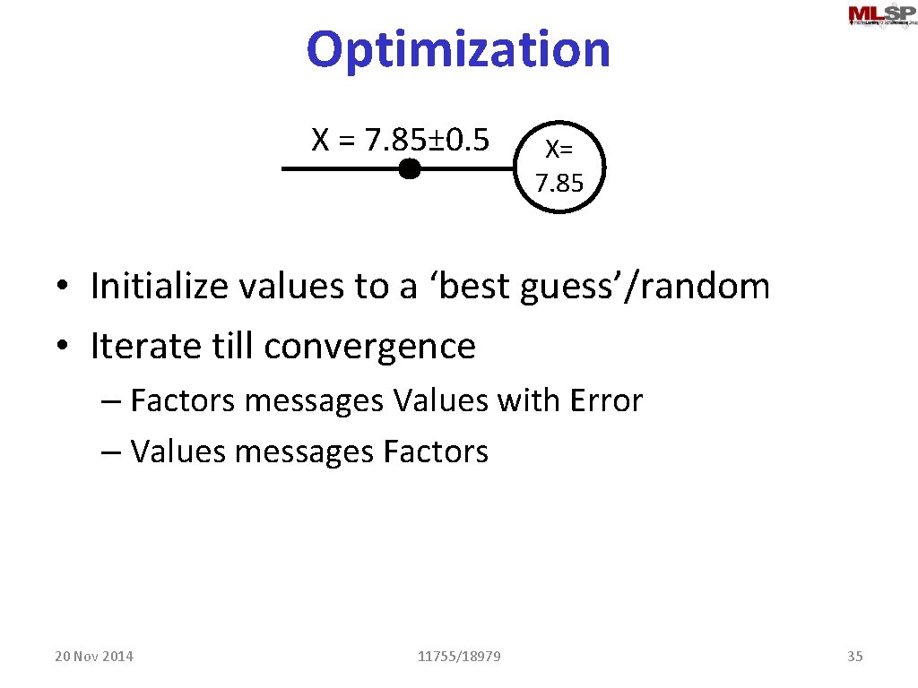
Optimization X = 7. 85± 0. 5 X= 7. 85 • Initialize values to a ‘best guess’/random • Iterate till convergence – Factors messages Values with Error – Values messages Factors 20 Nov 2014 11755/18979 35

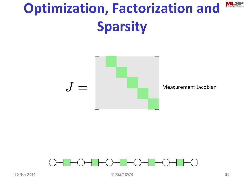
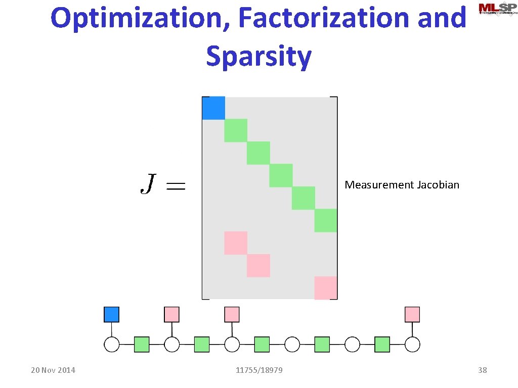
Optimization, Factorization and Sparsity Measurement Jacobian 20 Nov 2014 11755/18979 36

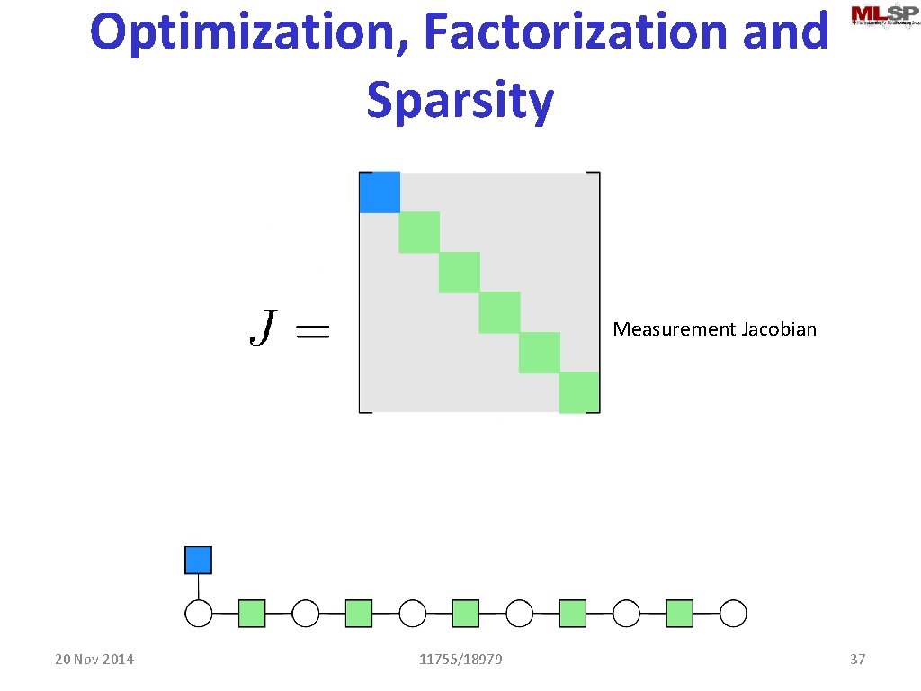
Optimization, Factorization and Sparsity Measurement Jacobian 20 Nov 2014 11755/18979 37

Optimization, Factorization and Sparsity Measurement Jacobian 20 Nov 2014 11755/18979 38

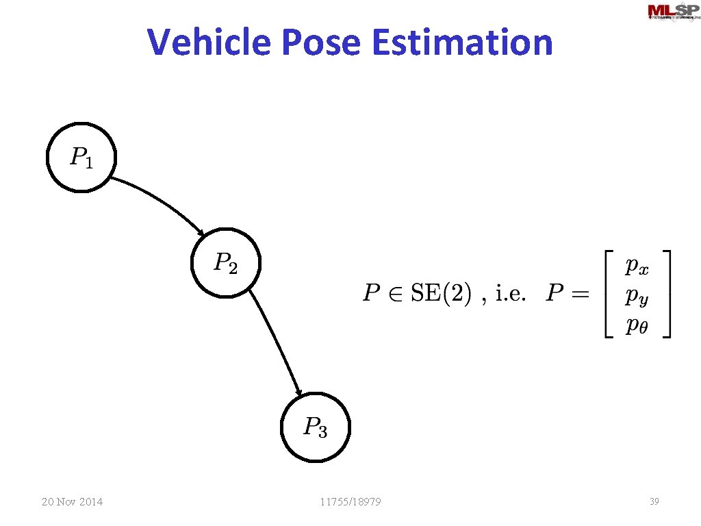
Vehicle Pose Estimation 20 Nov 2014 11755/18979 39

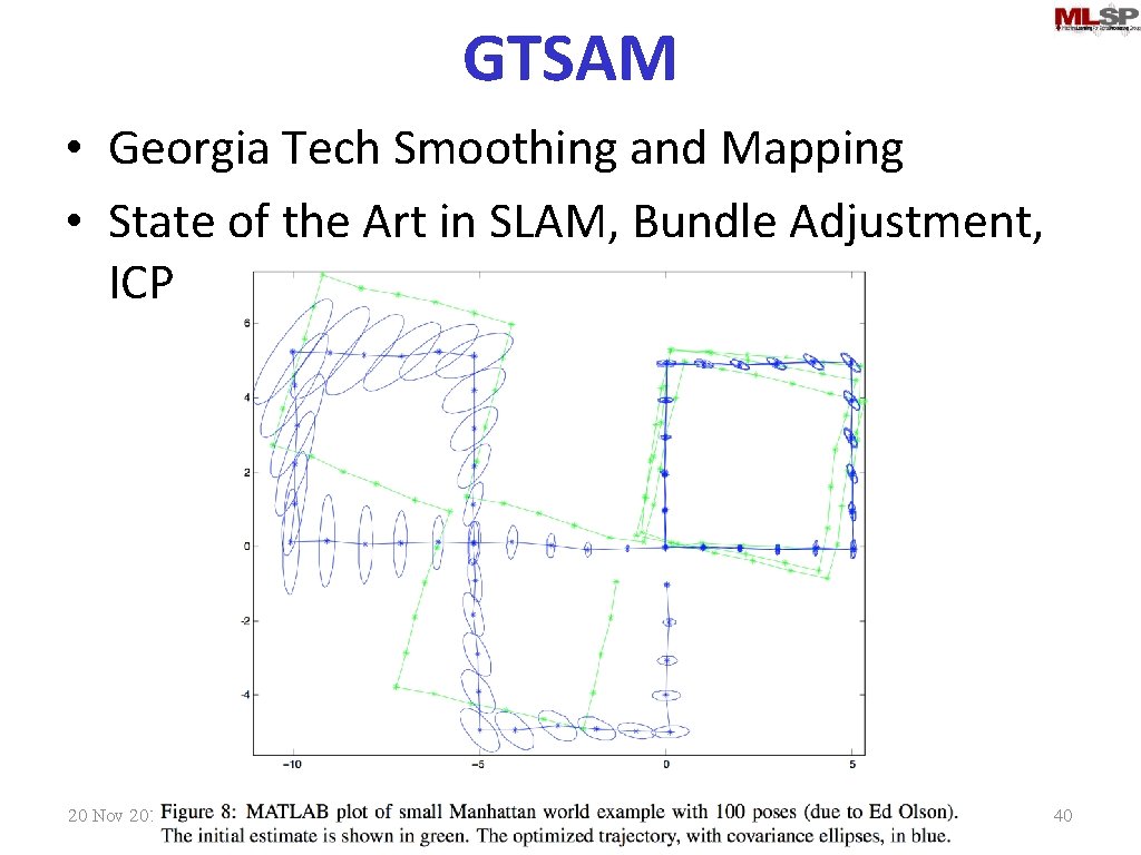
GTSAM • Georgia Tech Smoothing and Mapping • State of the Art in SLAM, Bundle Adjustment, ICP 20 Nov 2014 11755/18979 40

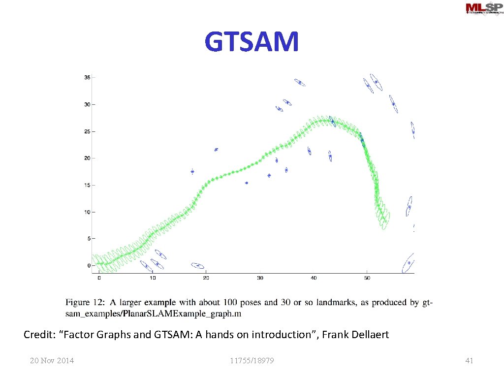
GTSAM Credit: “Factor Graphs and GTSAM: A hands on introduction”, Frank Dellaert 20 Nov 2014 11755/18979 41

SLAM versus Localization • No “landmarks”, rather just GPS readings • Odometry is modeled via similar means • Vehicle Model is far more constrained in comparison to a typical robotic agent

ARRB Vehicle Introduction • GPS @ 1 Hz • Gyroscope, Acceleration, Odometry @ 2. 0 meters – 2 -axis gyro and 2 -D accel leading to somewhat under constrained problem • Images @ 2. 0 -5. 0 meters (unsynchronised to above) • Random Noise including non-real-time OS errors so unrestrained arbitrary corruption of the data is possible! 43

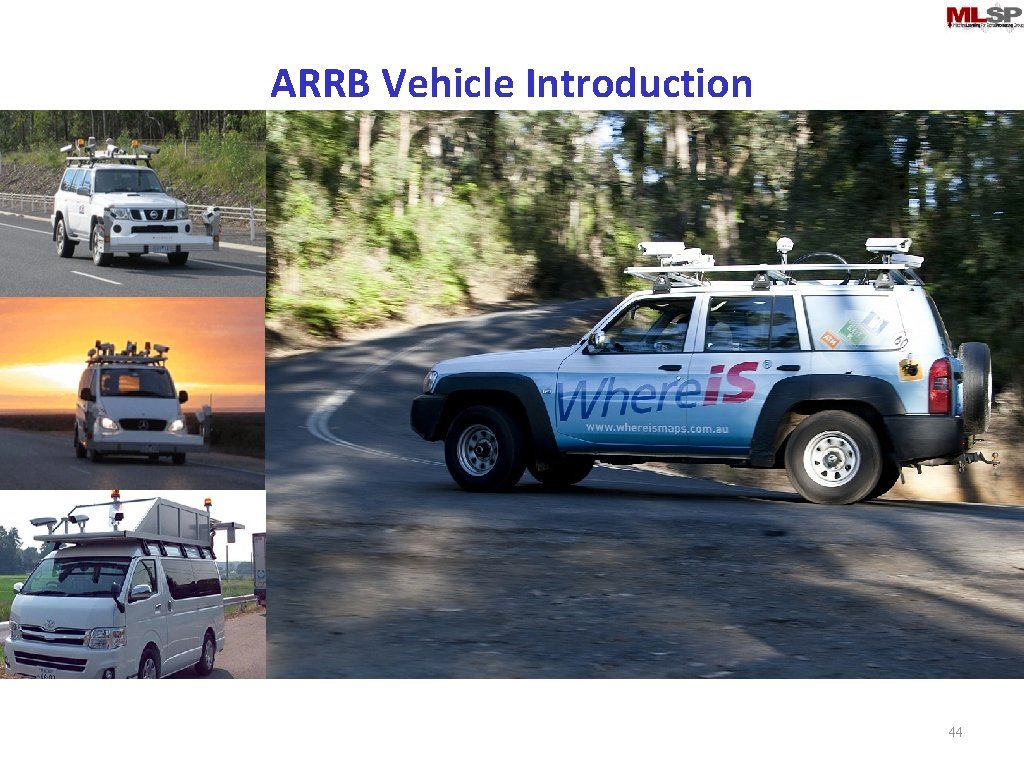
ARRB Vehicle Introduction 44

ARRB Vehicle Introduction • GPS @ 1 Hz • Gyroscope, Acceleration, Odometry @ 2. 0 meters – 2 -axis gyro and 2 -D accel leading to somewhat under constrained problem • Images @ 2. 0 -5. 0 meters (unsynchronised to above) • Random Noise including non-real-time OS errors so unrestrained arbitrary corruption of the data is possible! • This is the kind of great research problem that comes about on the back of greatly incompetent design! 45

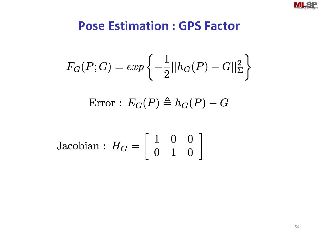
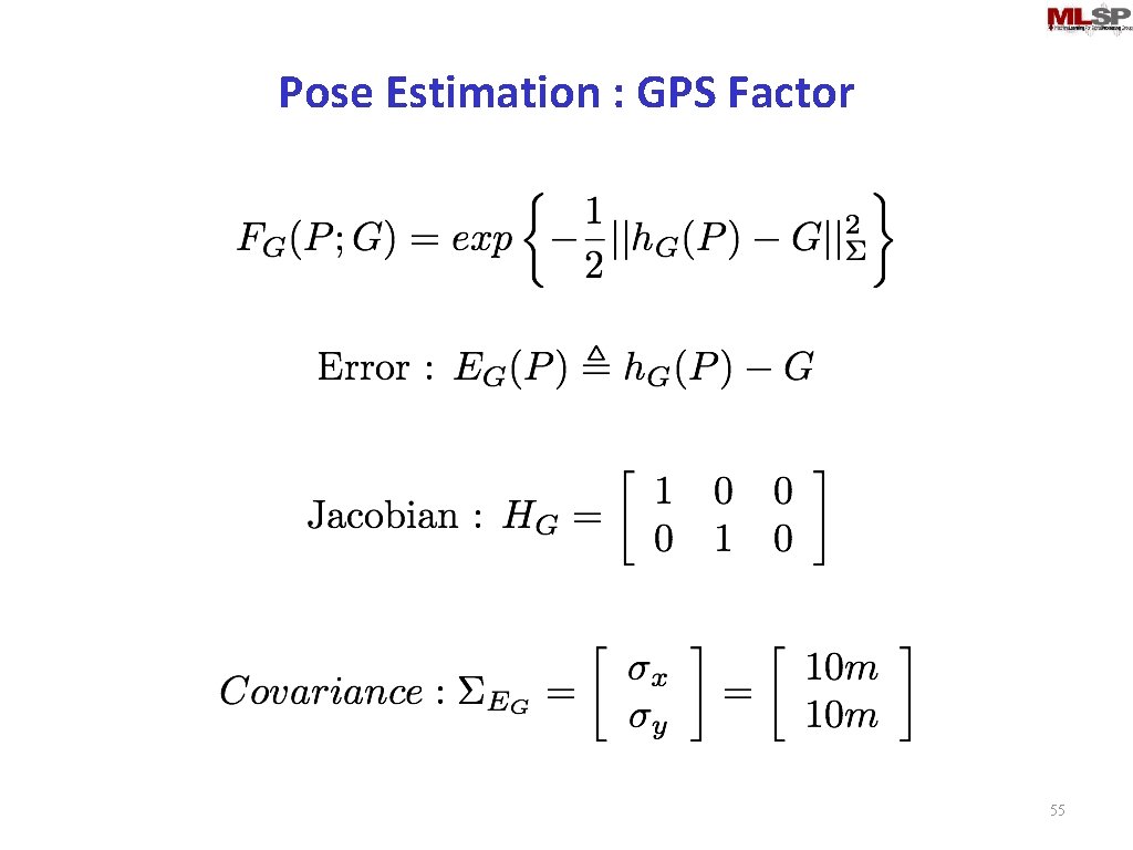
Pose Estimation : GPS Factor 46

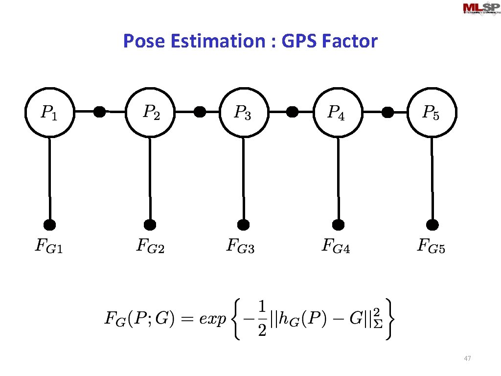
Pose Estimation : GPS Factor 47

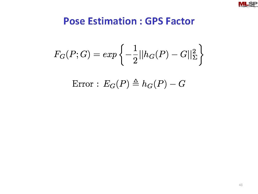
Pose Estimation : GPS Factor 48

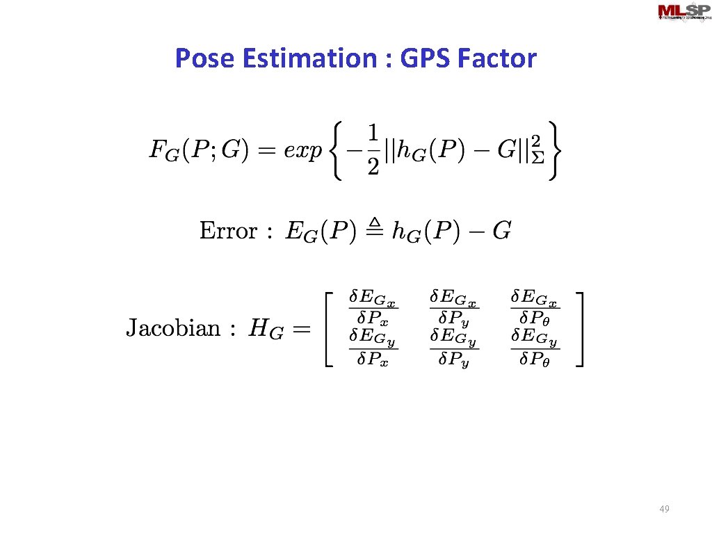
Pose Estimation : GPS Factor 49

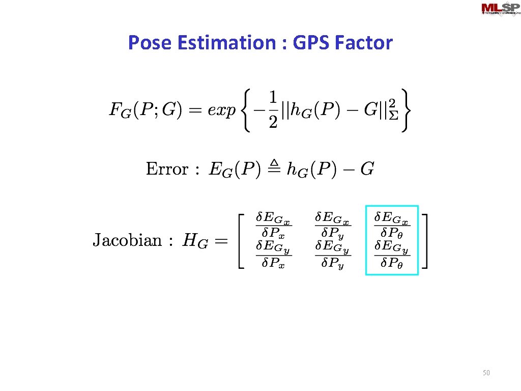
Pose Estimation : GPS Factor 50

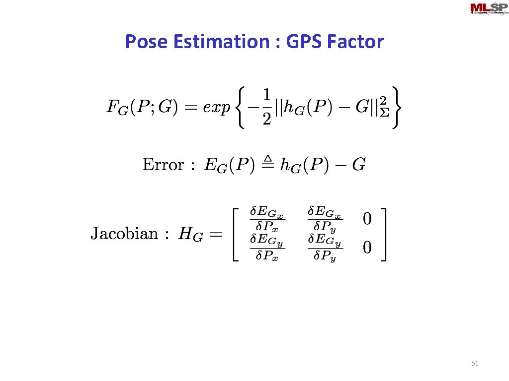
Pose Estimation : GPS Factor 51

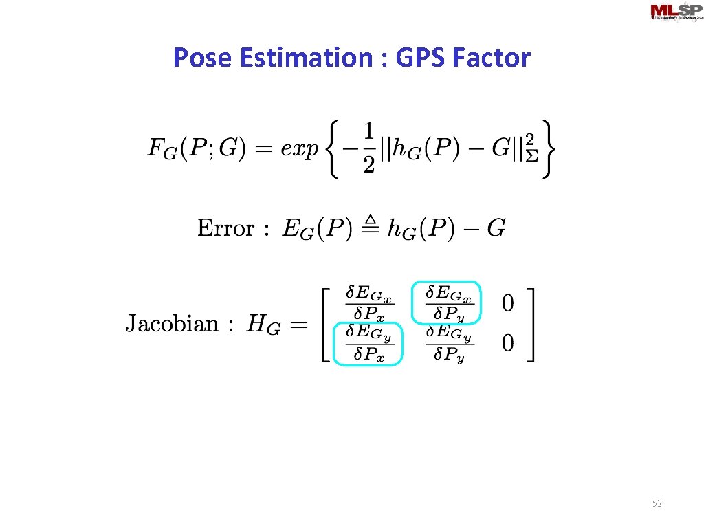
Pose Estimation : GPS Factor 52

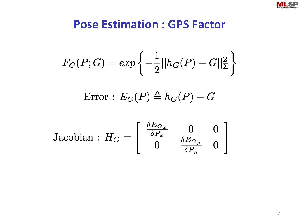
Pose Estimation : GPS Factor 53

Pose Estimation : GPS Factor 54

Pose Estimation : GPS Factor 55

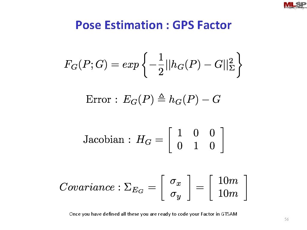
Pose Estimation : GPS Factor Once you have defined all these you are ready to code your Factor in GTSAM 56

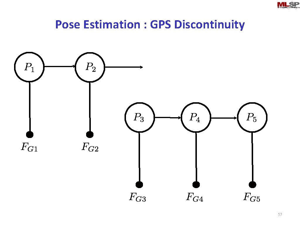
Pose Estimation : GPS Discontinuity 57

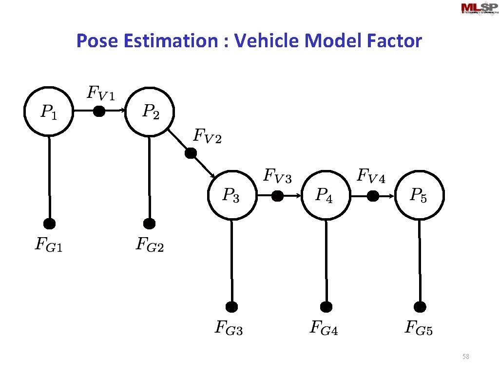
Pose Estimation : Vehicle Model Factor 58

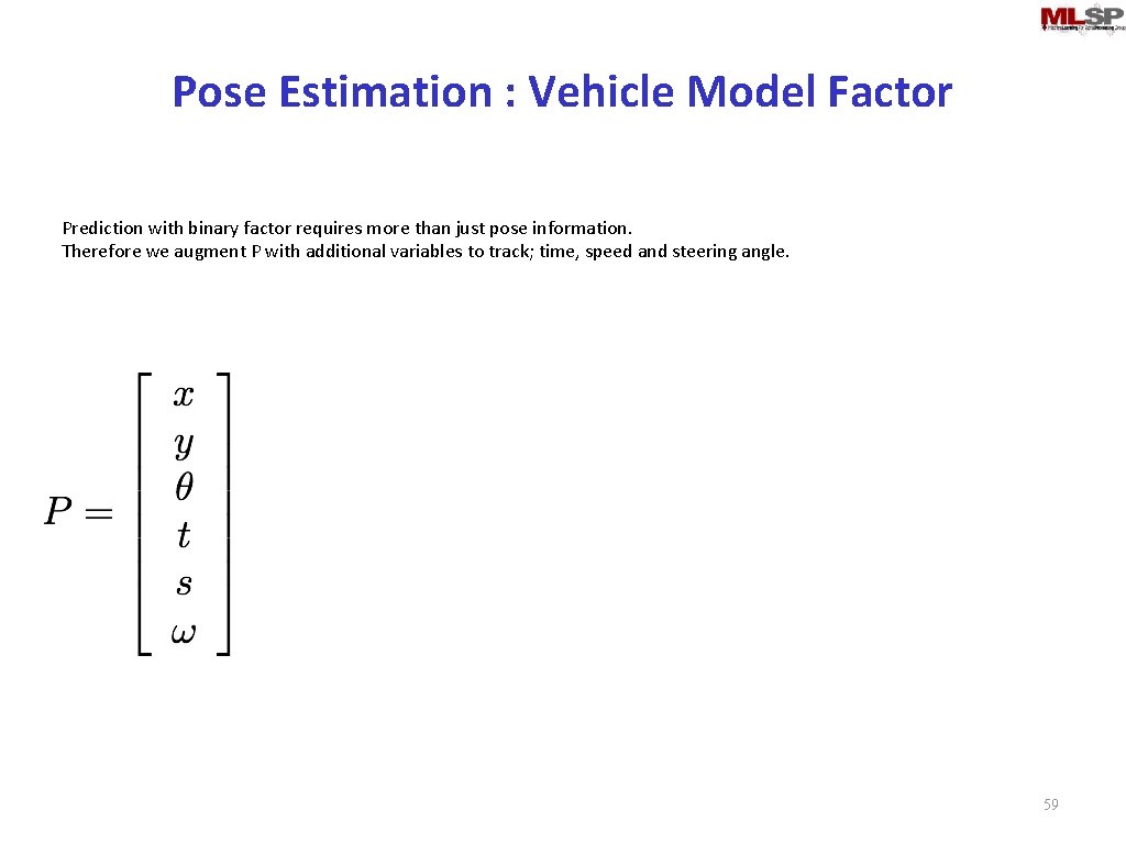
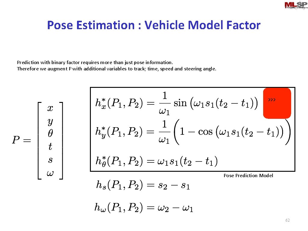
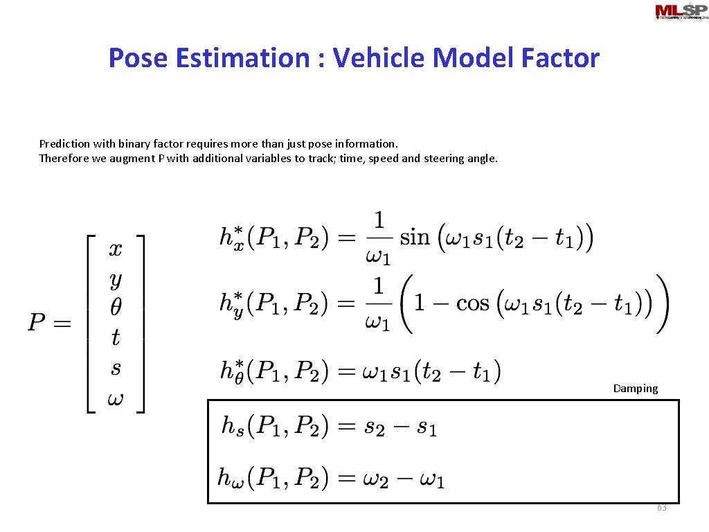
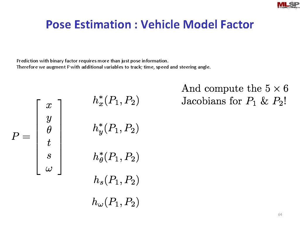
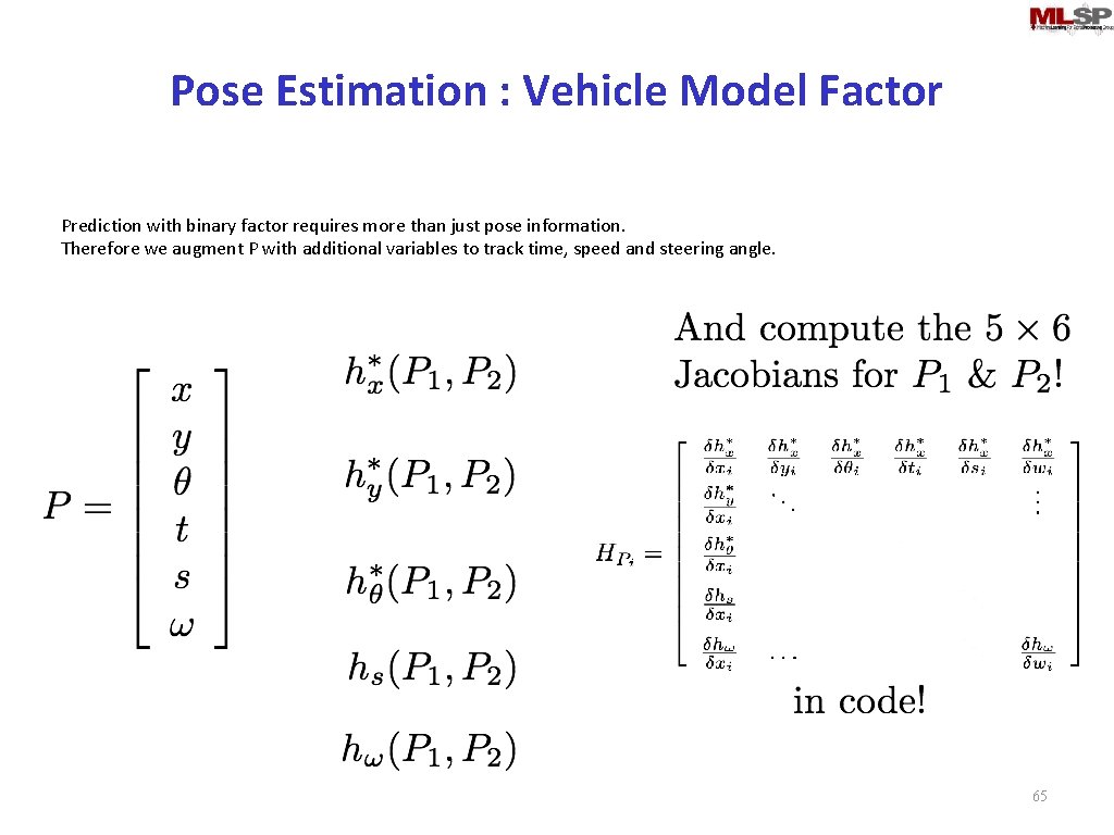
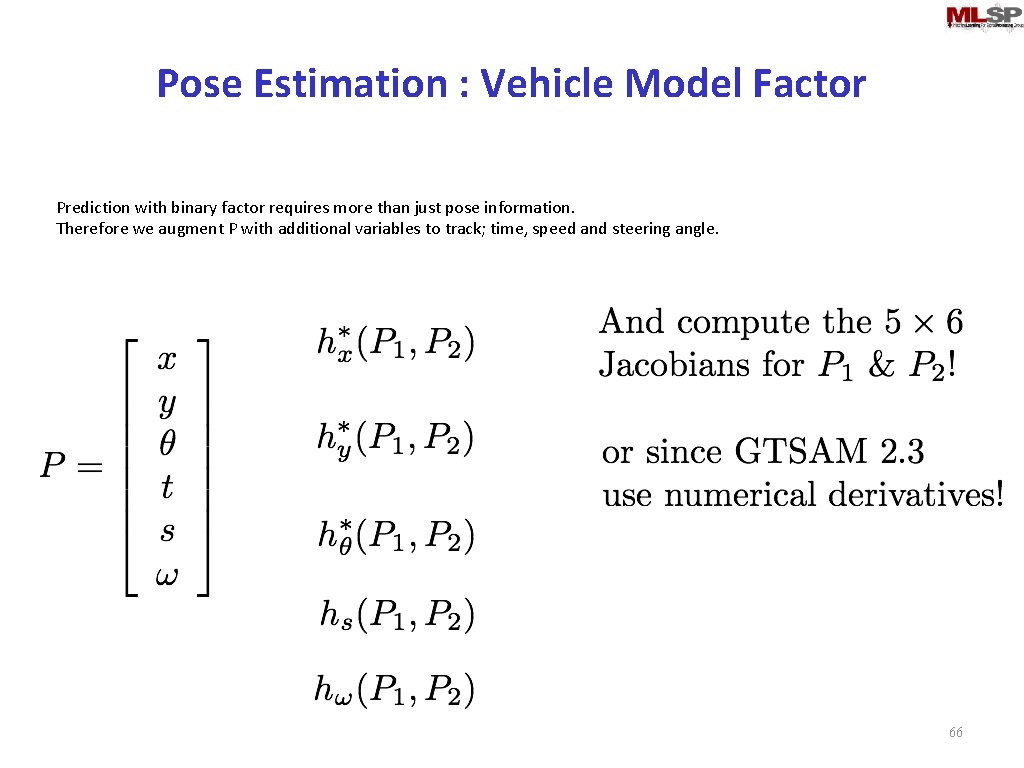
Pose Estimation : Vehicle Model Factor Prediction with binary factor requires more than just pose information. Therefore we augment P with additional variables to track; time, speed and steering angle. 59

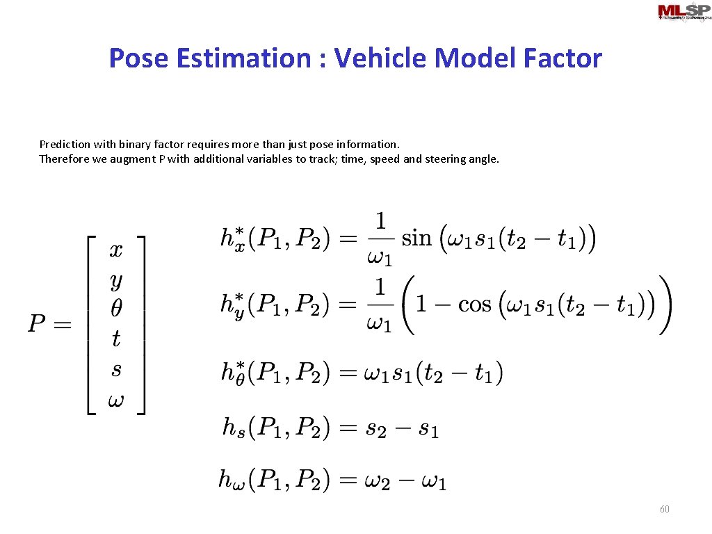
Pose Estimation : Vehicle Model Factor Prediction with binary factor requires more than just pose information. Therefore we augment P with additional variables to track; time, speed and steering angle. 60

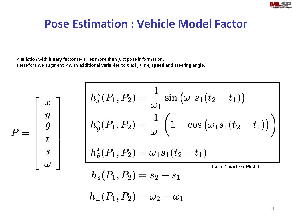
Pose Estimation : Vehicle Model Factor Prediction with binary factor requires more than just pose information. Therefore we augment P with additional variables to track; time, speed and steering angle. Pose Prediction Model 61

Pose Estimation : Vehicle Model Factor Prediction with binary factor requires more than just pose information. Therefore we augment P with additional variables to track; time, speed and steering angle. ? ? ? Pose Prediction Model 62

Pose Estimation : Vehicle Model Factor Prediction with binary factor requires more than just pose information. Therefore we augment P with additional variables to track; time, speed and steering angle. Damping 63

Pose Estimation : Vehicle Model Factor Prediction with binary factor requires more than just pose information. Therefore we augment P with additional variables to track; time, speed and steering angle. 64

Pose Estimation : Vehicle Model Factor Prediction with binary factor requires more than just pose information. Therefore we augment P with additional variables to track time, speed and steering angle. 65

Pose Estimation : Vehicle Model Factor Prediction with binary factor requires more than just pose information. Therefore we augment P with additional variables to track; time, speed and steering angle. 66

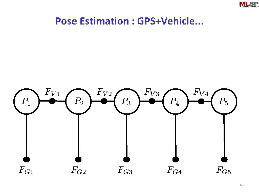
Pose Estimation : GPS+Vehicle. . . 67

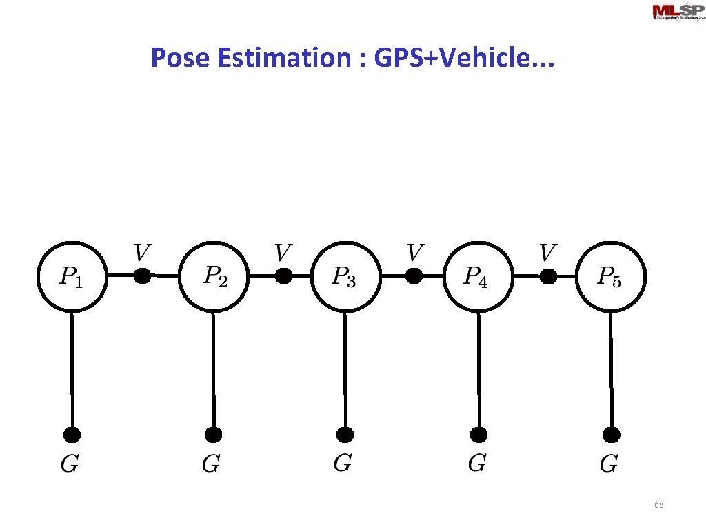
Pose Estimation : GPS+Vehicle. . . 68

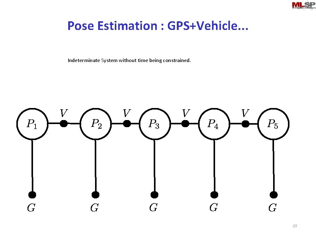
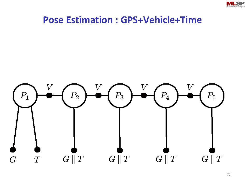
Pose Estimation : GPS+Vehicle. . . Indeterminate System without time being constrained. 69

Pose Estimation : GPS+Vehicle+Time 70

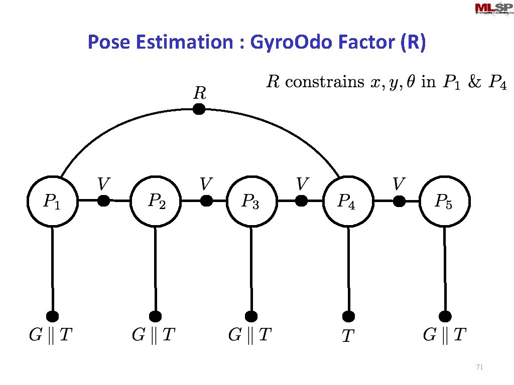
Pose Estimation : Gyro. Odo Factor (R) 71

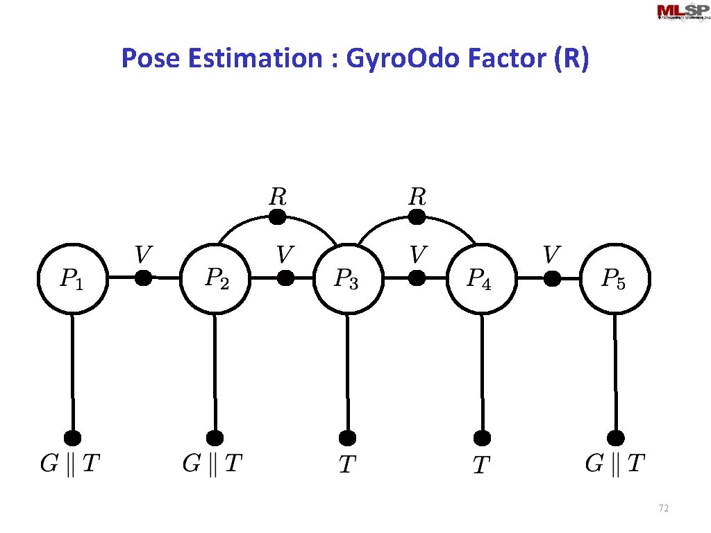
Pose Estimation : Gyro. Odo Factor (R) 72

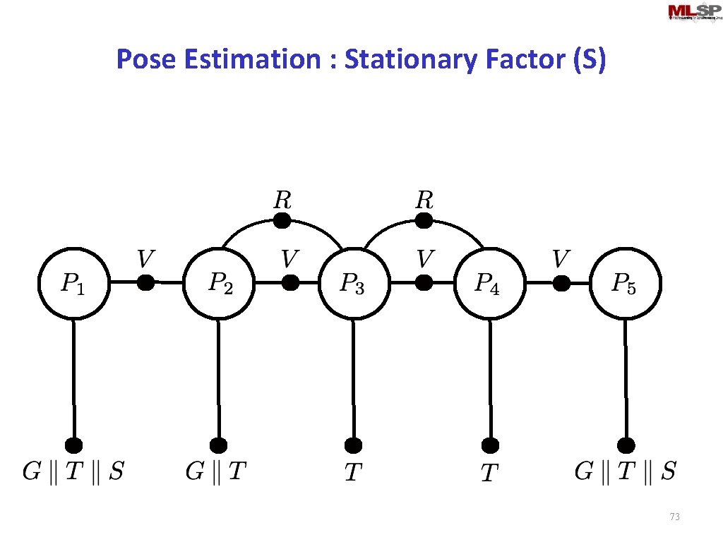
Pose Estimation : Stationary Factor (S) 73

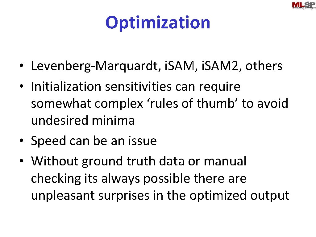
Optimization • Levenberg-Marquardt, i. SAM 2, others • Initialization sensitivities can require somewhat complex ‘rules of thumb’ to avoid undesired minima • Speed can be an issue • Without ground truth data or manual checking its always possible there are unpleasant surprises in the optimized output

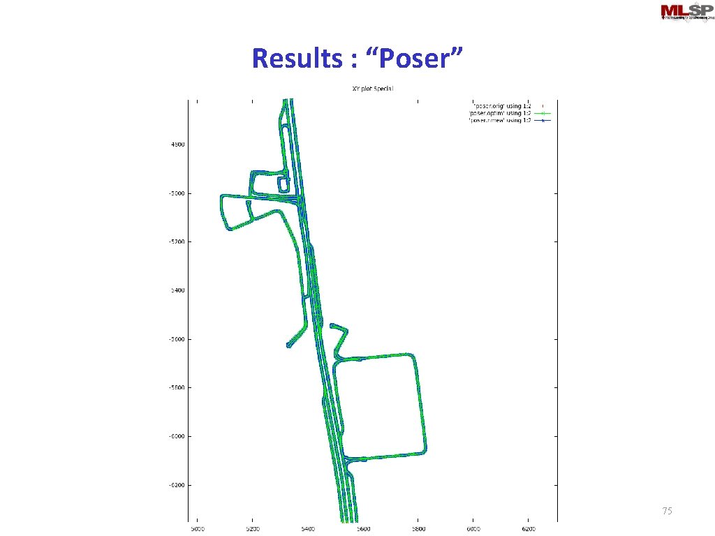
Results : “Poser” From imagination to impact 75

Results : “Poser” - more than 2 mile dropout 76

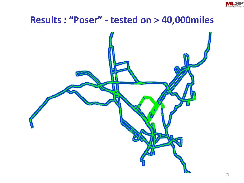
Results : “Poser” - tested on > 40, 000 miles 77

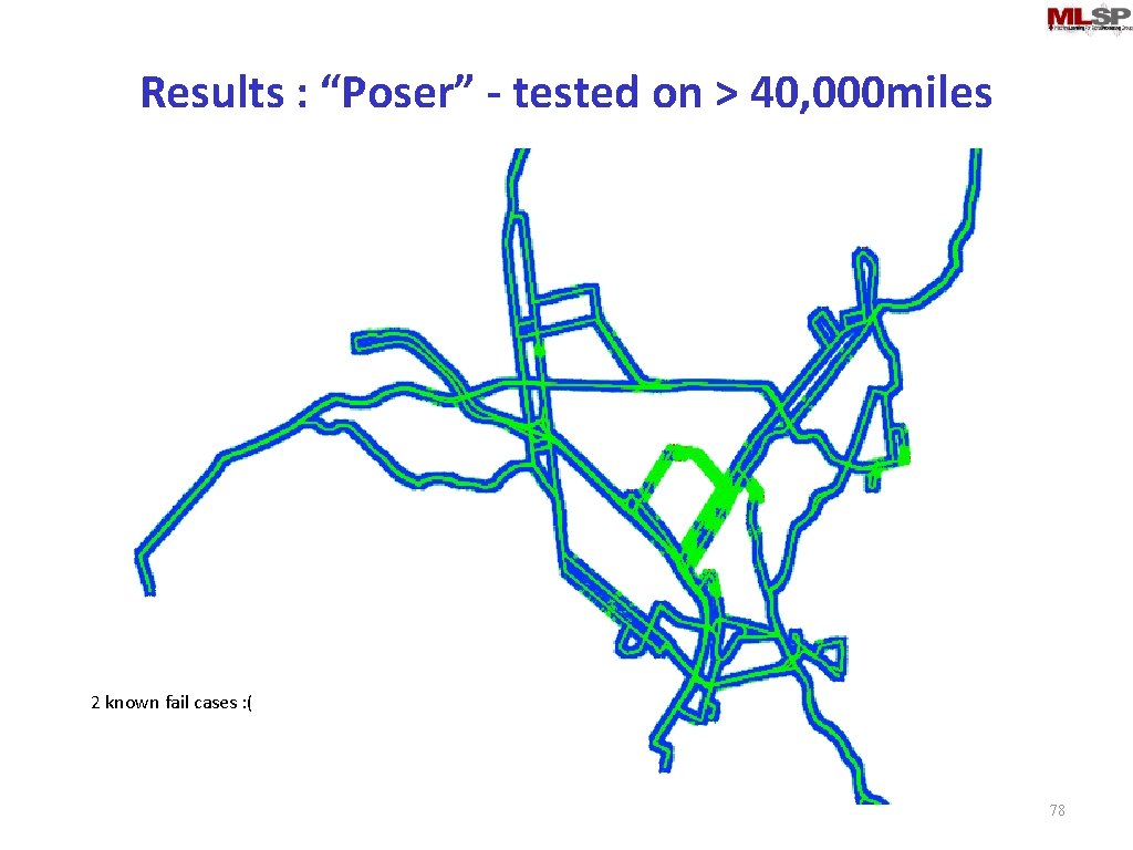
Results : “Poser” - tested on > 40, 000 miles 2 known fail cases : ( 78

GICP : Kinect Sensor https: //www. youtube. com/watch? v=TY 99 Y_I_egg 20 Nov 2014 11755/18979 79

Factor Graphs : Round Up • Factor Graphs are great for expressing formally defined relationships (e. g. in SLAM we ‘know’ how GPS positions should relate to real world locations) • Highly General Tool – but its useful for building specific models/capturing prior knowledge you can formalize • Contrast with Neural Networks – both are graphical models but Neural Networks work to discover the unknown (or you are lazy) relationships as opposed to known ones. 80

Resources • GTSAM - https: //collab. cc. gatech. edu/borg/download • “Factor Graphs and GTSAM: A hands on introduction”, Frank Dellaert • Michael Kaess – GTSAM contributor now at CMU-RI (see https: //www. ri. cmu. edu/video_view. html? video_id=129&menu_id=387) • G 2 O – an alternative library for similar factor graph optimizations • Dimple – Graphical Modelling Tool http: //dimple. probprog. org/ 81