Markov Model Markov Model Markov Chain Firstorder Markov

Markov Model • Markov Model (Markov Chain) – First-order Markov chain of N states is a triplet (S, A, ) S is a set of N states • A is the N N matrix of state transition probabilities P(qt=j|qt-1=i, qt-2=k, ……)=P (qt=j|qt-1=i) aij • is the vector of initial state probabilities j =P(q 0=j) • – The output for any given state is an observable event (deterministic) – The output of the process is a sequence of observable events A Markov chain with 5 states (labeled S 1 to S 5) with state transitions. 2

Markov Model • An example : a 3 -state Markov Chain λ – State 1 generates symbol A only, State 2 generates symbol B only, and State 3 generates symbol C only 0. 6 s 1 0. 3 0. 7 s 2 B A 0. 3 0. 1 0. 2 s 3 0. 7 C – Given a sequence of observed symbols O={CABBCABC}, the only one corresponding state sequence is {S 3 S 1 S 2 S 2 S 3 S 1 S 2 S 3}, and the corresponding probability is P(O|λ)=P(q 0=S 3) P(S 1|S 3)P(S 2|S 1)P(S 2|S 2)P(S 3|S 2)P(S 1|S 3)P(S 2|S 1)P(S 3|S 2) =0. 1 0. 3 0. 7 0. 2 0. 3 0. 2=0. 00002268 3

Hidden Markov Model • HMM, an extended version of Markov Model – The observation is a probabilistic function (discrete or continuous) of a state instead of an one-to-one correspondence of a state – The model is a doubly embedded stochastic process with an underlying stochastic process that is not directly observable (hidden) • What is hidden? The State Sequence According to the observation sequence, we never know which state sequence generates it • Elements of an HMM {S, A, B, } – S is a set of N states – A is the N N matrix of state transition probabilities – B is a set of N probability functions, each describing the observation probability with respect to a state – is the vector of initial state probabilities 4

Simplified HMM 1 2 3 RGBGGBBGRRR…… 5

Hidden Markov Model • Two types of HMM’s according to the observation functions Discrete and finite observations : – The observations that all distinct states generate are finite in number V={v 1, v 2, v 3, ……, v. M}, vk RD – the set of observation probability distributions B={bj(vk)} is defined as bj(vk)=P(ot=vk|qt=j), 1 k M, 1 j N ot : observation at time t, qt : state at time t for state j, bj(vk) consists of only M probability values Continuous and infinite observations : – The observations that all distinct states generate are infinite and continuous, V={v| v RD} – the set of observation probability distributions B={bj(v)} is defined as bj(v)=P (ot=v|qt=j), 1 j N bj(v) is a continuous probability density function and is often assumed to be a mixture of Gaussian distributions 6

Hidden Markov Model • An example : a 3 -state discrete HMM λ 0. 6 s 1 0. 3 0. 7 s 2 {A: . 3, B: . 2, C: . 5} 0. 3 0. 1 0. 2 s 3 0. 7 {A: . 7, B: . 1, C: . 2} {A: . 3, B: . 6, C: . 1} – Given a sequence of observations O={ABC}, there are 27 possible corresponding state sequences, and therefore the corresponding probability is 7

Hidden Markov Model • Three Basic Problems for HMMs Given an observation sequence O=(o 1, o 2, …. . , o. T), and an HMM λ =(A, B, ) – Problem 1 : How to efficiently compute P(O| λ) ? Evaluation problem – Problem 2 : How to choose an optimal state sequence q=(q 1, q 2, ……, q. T) ? Decoding Problem – Problem 3 : Given some observations O for the HMM λ , how to adjust the model parameter λ =(A, B, ) to maximize P(O| λ)? Learning /Training Problem 8

Basic Problem 1 for HMM 1 2 N = (A, B, p) O = o 1 o 2 o 3……ot……o. T observation sequence q = q 1 q 2 q 3……qt……q. T state sequence ․Problem 1: Given and O, find P(O| )=Prob[observing O given ] ․Direct Evaluation: considering all possible state sequence q all q P(O | q, ) P(O| ) = ([bq 1(o 1) bq 2(o 2) ……bq. T(o. T)] all q [pq 1 aq 1 q 2 aq 2 q 3 ……aq. T-1 q. T]) P(q| ) T total number of different q : N huge computation requirements 9

10

Basic Problem 1 3 2 1 11

Basic Problem 1 αt(i) = P(o 1 o 2……ot , qt = i| ) i t t 12

Basic Problem 1 αt+1(j) N t+1( j) = [ t(i)aij ] bj(ot+1) i=1 j i 1 j N 1 t T 1 αt(i) t t+1 Forward Algorithm 13

14

Basic Problem 2 t(i) = P(ot+1 , ot+2 , …, o. T |qt= i, ) βt(i) i t T t+1 15

Basic Problem 2 βt+1(j) βt(i) N t( i) = aij bj(ot+1) t+1( j) j=1 t = T 1, T 2, …, 2, 1, 1 i N j i t t+1 T Backward Algorithm 16

Basic Problem 2 βt(i) i P(O, qt = i | ) = Prob [observing o 1, o 2, …, ot , …, o. T , qt = i | ] αt(i) t = t(i) 17

Basic Problem 2 N N i=1 P(O| ) = P(O, qt = i | ) = [ t(i)] P(Ō|λ) αt(i)βt(i) i t N P(O| ) = T(i) i=1 18

Basic Problem 2 for HMM ․Approach 1 – Choosing state q t* individually as the most likely state at time t - Define a new variable t(i) = P(qt = i | O, ) P(O, qt= i| ) t(i) = = N P(O| ) t(i) i=1 - Solution qt* = arg max [ t(i)], 1 t T 1£ i £ N in fact qt* = arg max [P(O, qt= i| )] 1£ i £ N = arg max [ t(i)] 1£ i £ N - Problem maximizing the probability at each time t individually q*= q 1*q 2*…q. T* may not be a valid sequence (e. g. aqt*qt+1* = 0) 19

20

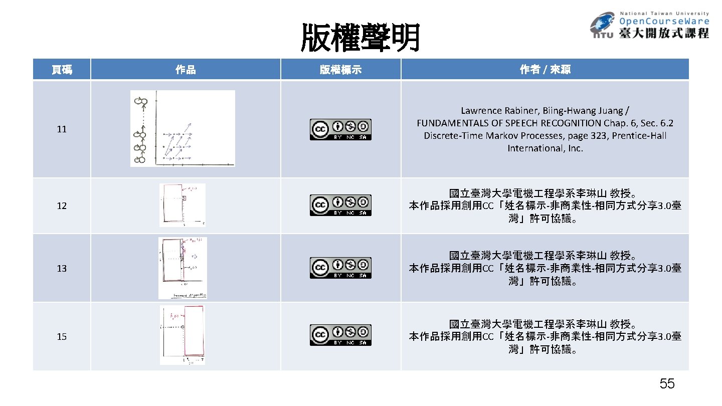
Viterbi Algorithm t+1( j) = max [ t(i)aij] bj(ot+1) i i δt(i) δt+1(j) j i δt(i) 1 1 t t(i) = max P[q 1, q 2, …qt-1, qt = i, o 1, o 2, …, ot | ] q 1, q 2, …q t t+1 t-1 21

Viterbi Algorithm Path backtracking 22

23

Basic Problem 2 for HMM ․Application Example of Viterbi Algorithm - Isolated word recognition. . . observation 1£ i £ n 24 1£ i £ n Problem 2 Basic Problem Basic 1 Viterbi Algorithm Forward Algorithm (for single best path) for the most probable pa all with paths) -The (for model theahighest probability usually also has the highest probability for all possible paths. 24

25

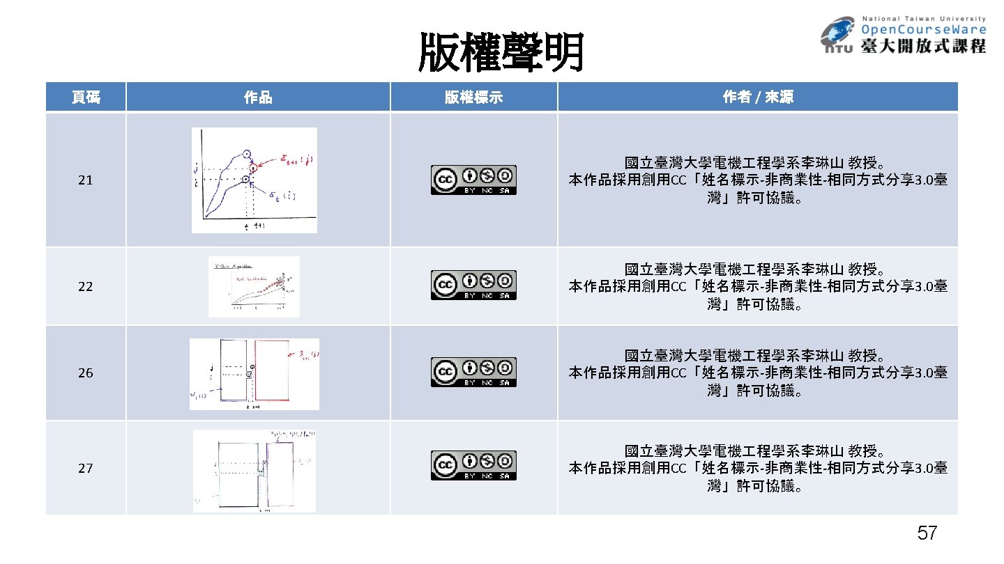
Basic Problem 3 t(i) aij bj(ot+1) t+1( j) βt+1(j) j i αt(i) t t+1 26

Basic Problem 3 αt(i)aijbj(ot+1)βt+1(j) j i αt(i) t t+1 27

Basic Problem 3 28

Basic Problem 3 T-1 (i, j)/(T-1) t a ij = t. T-1 =1 (i)/(T-1) t t =1 29

30

31

32

Basic Problem 3 33

Basic Problem 3 34

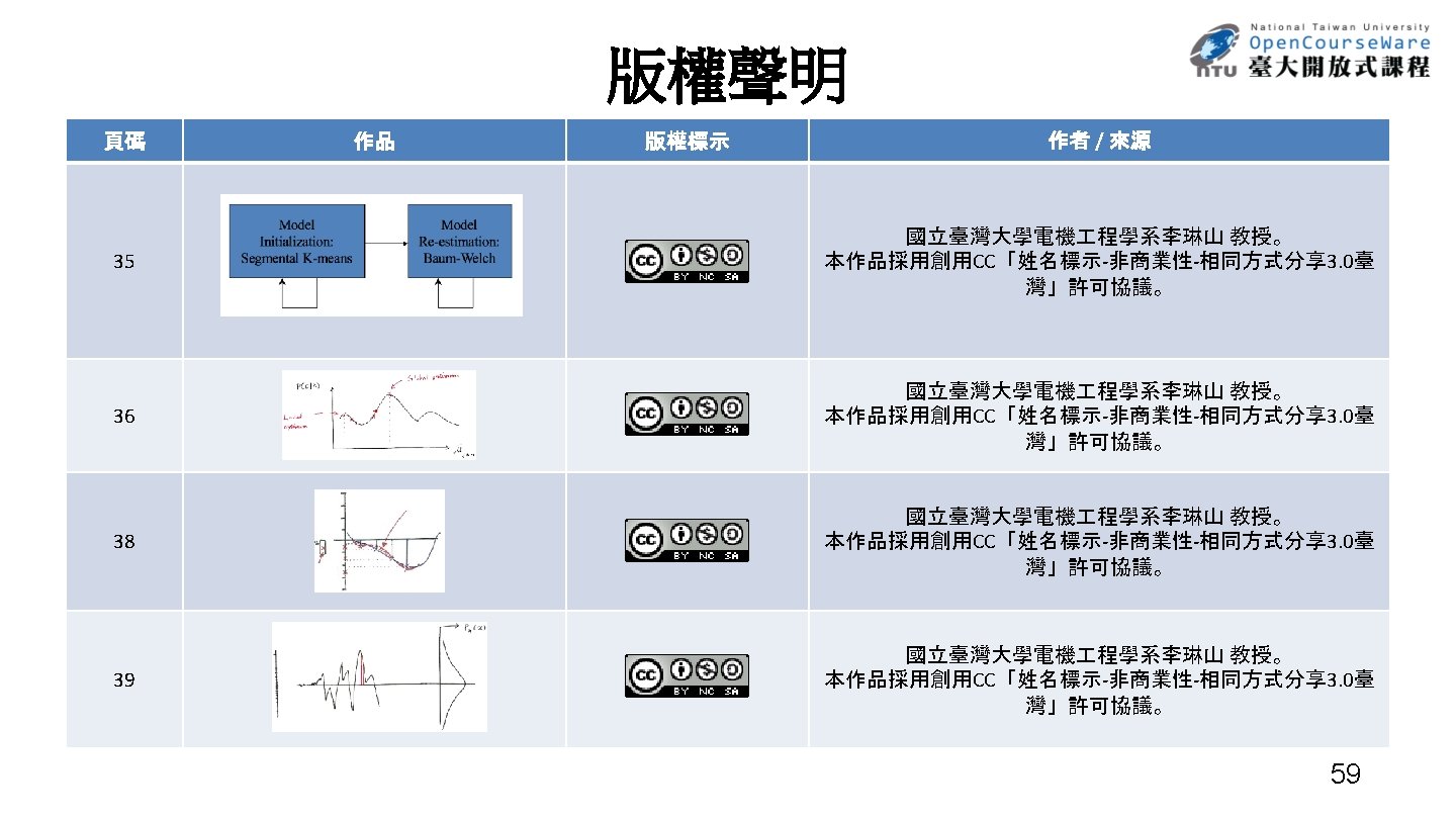
Basic Problem 3 for HMM l No closed-form solution, but approximated iteratively l An initial model is needed-model initialization l May converge to local optimal points rather than global optimal point - heavily depending on the initialization l Model training Model Initialization: Re-estimation: Segmental K-means Baum-Welch 35

Basic Problem 3 P(O|λ) P Global optimum Local optimum jkn 36

Vector Quantization (VQ) • An Efficient Approach for Data Compression – replacing a set of real numbers by a finite number of bits • An Efficient Approach for Clustering Large Number of Sample Vectors – grouping sample vectors into clusters, each represented by a single vector (codeword) • Scalar Quantization – replacing a single real number by an R-bit pattern – a mapping relation Jk A=m S= J vk A= m } L –Quantization characteristics (codebook) , V ={ v 1 , v 2 , …, v. L { J 1 , J 2 , …, JL } and { v 1 , v 2 , …, v. L Q 0 : S V } Q(x[n]) = vk if x[n] Jk designed considering at least L = 2 R Each vk represented by an R-bit pattern 1. error sensitivity 2. probability distribution of x[n] k 37

Vector Quantization Scalar Quantization ：Pulse Coded Modulation (PCM) 011 010 quantization error 001 000 101 110 111 100 101 110 38

Vector Quantization Px(x) 39

Vector Quantization (VQ) 2 -dim Vector Quantization (VQ) Example: xn = ( x[n] , x[n+1] ) S ={xn = (x[n] , x[n+1] ) ; |x[n]| <A, |x[n+1]|<A} • VQ –S divided into L 2 -dim regions { J 1 , J 2 , …, Jk , …JL } – Considerations 1. error sensitivity may depend on x[n], x[n+1] jointly 2. distribution of x[n] , x[n+1] may be correlated statistically 3. more flexible choice of Jk each with a representative vector vk Jk, V= { v 1 , v 2 , …, v. L } –Q : S V – Quantization Characteristics Q(xn)= vk if xn Jk (codebook) L = 2 R { J 1 , J 2 , …, JL } and { v 1 , v 2 , …, v. L } each vk represented by an R-bit pattern 40

Vector Quantization 41

Vector Quantization Jk vk 2 8 2 (256) =(2 ) =2 1024=2 10 16 42

Vector Quantization Jk vk 43

Vector Quantization (VQ) N-dim Vector Quantization x = (x 1 , x 2 , …, x. N ) S = {x = (x 1 , x 2 , …, x. N) , | xk |< A , k = 1, 2, …N} V = {v 1 , v 2 , …, v. L } Q: S V Q(x) = vk if x Jk L = 2 R , each vk represented by an R-bit pattern Codebook Trained by a Large Training Set ˙Define distance measure between two vectors x, y d( x, y ) : S S R+ (non-negative real numbers) -desired properties d( x, y ) 0 d( x, x ) = 0 d( x, y ) = d( y, x ) d( x, y ) + d( y, z ) d( x, z ) examples : d( x, y ) = (xi yi)2 i d( x, y ) = | xi yi | i d( x, y ) = (x-y)t -1(x-y) Mahalanobis Distance : Co-variance Matrix 44

Distance Measures city block distance Mahalanobis distance 45

Vector Quantization (VQ) • K-Means Algorithm/Lloyd-Max Algorithm (2) (1) Fixed { J 1 , J 2 , …, JL } find best set of Fixed { v 1 , v 2 , …, v. L } find best set of J 1 , , Jv 2 , )…, JL }, v (3) (1) Jk = { x |{d(x < d(x condition k j) Convergence L , j k} D = Dk D = d(x , Q(x) ) = min after each iteration D is reduced, but D 0 nearest neighbor | D(m+1) D(m) | < , m : condition iteration • Iterative Procedure to Obtain Codebook from a Large Training Set (2) For each k k=1 46

Vector Quantization 47

Vector Quantization (VQ) • K-means Algorithm may Converge to Local Optimal Solutions – depending on initial conditions, not unique in general • Training VQ Codebook in Stages― LBG Algorithm – step 1: Initialization. L = 1, train a 1 -vector VQ codebook – step 2: Splitting the L codewords into 2 L codewords, L = 2 L ‧example 1 ‧example 2 : the vector most far apart – step 3: k-means Algorithm: to obtain L-vector codebook – step 4: Termination. Otherwise go to step 2 • Usually Converges to Better Codebook 48

LBG Algorithm 49

Initialization in HMM Training • An Often Used Approach― Segmental K-Means – Assume an initial estimate of all model parameters (e. g. estimated by segmentation of training utterances into states with equal length) • For discrete density HMM • For continuous density HMM (M Gaussian mixtures per state) – Step 1 : re-segment the training observation sequences into states based on the initial model by Viterbi Algorithm – Step 2 : Reestimate the model parameters (same as initial estimation) – Step 3: Evaluate the model score P( |λ): If the difference between the previous and current model scores exceeds a threshold, go back to Step 1, otherwise stop and the initial model is obtained 50

Segmental K-Means 51

Initialization in HMM Training • An example for Continuous HMM – 3 states and 4 Gaussian mixtures per state State s 3 s 3 s 3 s 2 s 2 s 2 s 1 s 1 s 1 1 2 N O 1 O 2 ON { 12, c 12} { 11, c 11} LBG Global mean Cluster 1 mean Cluster 2 mean K-means { 13, c 13{ } 14, c 14} 52

Initialization in HMM Training • An example for discrete HMM – 3 states and 2 codewords State s 3 s 3 s 3 s 2 s 2 s 2 s 1 s 1 s 1 1 2 3 4 5 6 7 8 9 10 O 1 O 2 O 3 O 4 O 5 O 6 O 7 O 8 O 9 O 10 b 1(v 1)=3/4, b 1(v 2)=1/4 b 2(v 1)=1/3, b 2(v 2)=2/3 b 3(v 1)=2/3, b 3(v 2)=1/3 v 1 v 2 53