Markov Decision Processes II Tai Sing Lee 15

- Slides: 52

Markov Decision Processes II Tai Sing Lee 15 -381/681 AI Lecture 15 Read Chapter 17. 1 -3 of Russell & Norvig With thanks to Dan Klein, Pieter Abbeel (Berkeley), and Past 15 -381 Instructors for slide contents, particularly Ariel Procaccia, Emma Brunskill and Gianni Di Caro.

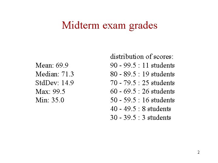
Midterm exam grades Mean: 69. 9 Median: 71. 3 Std. Dev: 14. 9 Max: 99. 5 Min: 35. 0 distribution of scores: 90 - 99. 5 : 11 students 80 - 89. 5 : 19 students 70 - 79. 5 : 25 students 60 - 69. 5 : 26 students 50 - 59. 5 : 16 students 40 - 49. 5 : 8 students 30 - 39. 5 : 3 students 2

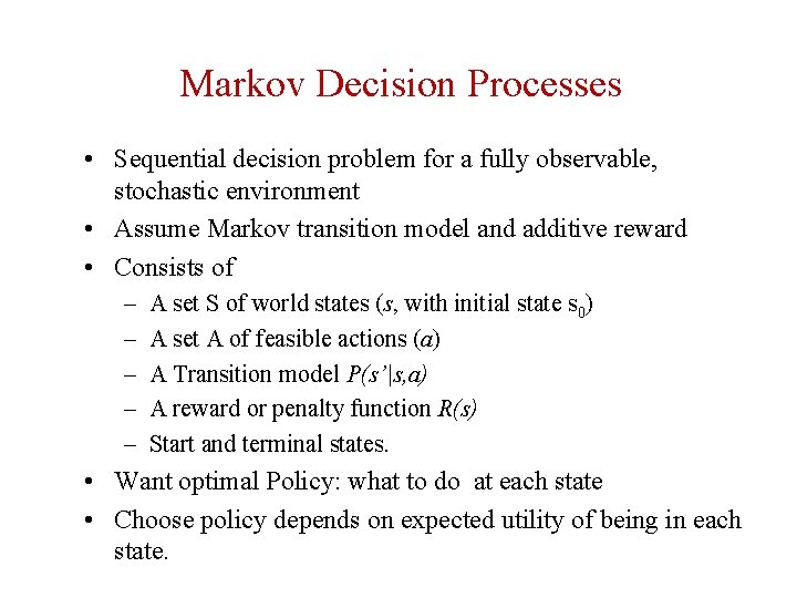
Markov Decision Processes • Sequential decision problem for a fully observable, stochastic environment • Assume Markov transition model and additive reward • Consists of – – – A set S of world states (s, with initial state s 0) A set A of feasible actions (a) A Transition model P(s’|s, a) A reward or penalty function R(s) Start and terminal states. • Want optimal Policy: what to do at each state • Choose policy depends on expected utility of being in each state.

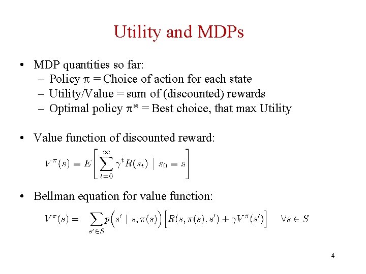
Utility and MDPs • MDP quantities so far: – Policy = Choice of action for each state – Utility/Value = sum of (discounted) rewards – Optimal policy * = Best choice, that max Utility • Value function of discounted reward: • Bellman equation for value function: 4

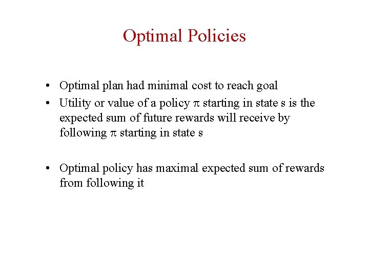
Optimal Policies • Optimal plan had minimal cost to reach goal • Utility or value of a policy starting in state s is the expected sum of future rewards will receive by following starting in state s • Optimal policy has maximal expected sum of rewards from following it

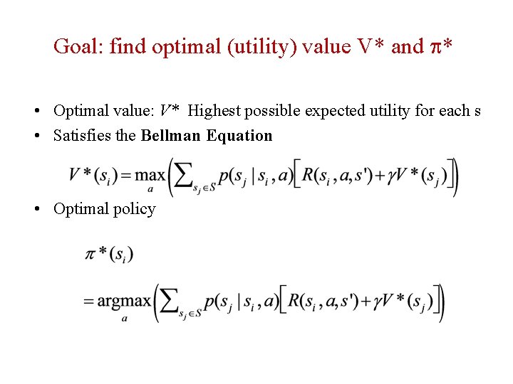
Goal: find optimal (utility) value V* and * • Optimal value: V* Highest possible expected utility for each s • Satisfies the Bellman Equation • Optimal policy

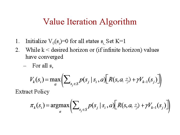
Value Iteration Algorithm 1. Initialize V 0(si)=0 for all states si, Set K=1 2. While k < desired horizon or (if infinite horizon) values have converged – For all s, Sj) Extract Policy Sj)

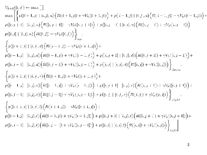
8

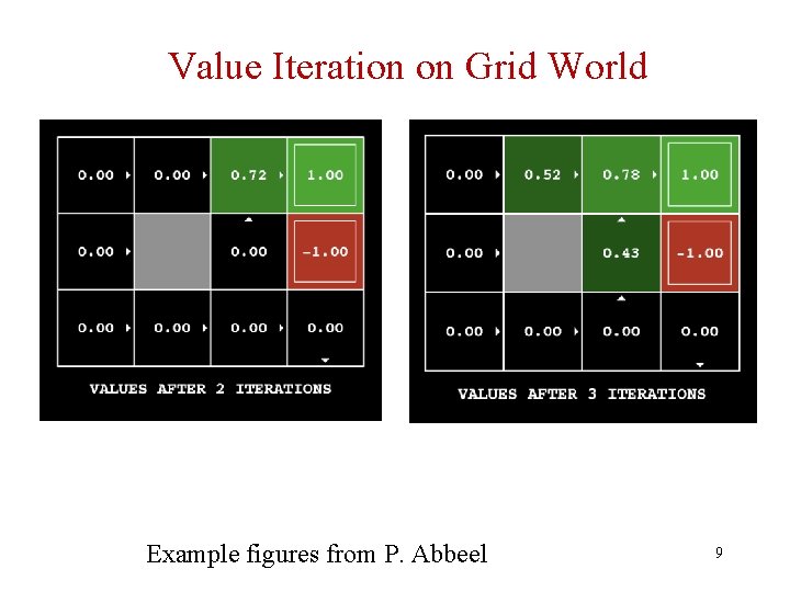
Value Iteration on Grid World Example figures from P. Abbeel 9

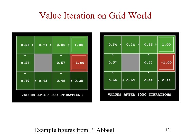
Value Iteration on Grid World Example figures from P. Abbeel 10

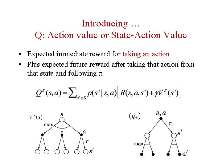
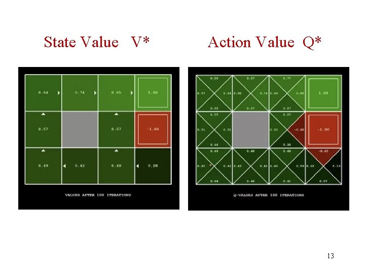
Introducing … Q: Action value or State-Action Value • Expected immediate reward for taking an action • Plus expected future reward after taking that action from that state and following

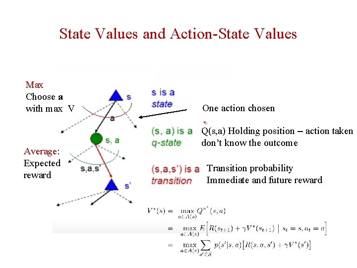
State Values and Action-State Values Max Choose a with max V Average: Expected reward One action chosen Q(s, a) Holding position – action taken don’t know the outcome Transition probability Immediate and future reward

State Value V* Action Value Q* 13

14

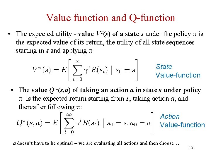
Value function and Q-function • The expected utility - value V (s) of a state s under the policy is the expected value of its return, the utility of all state sequences starting in s and applying State Value-function • The value Q (s, a) of taking an action a in state s under policy is the expected return starting from s, taking action a, and thereafter following : Action Value-function a doesn’t have to be optimal – we are evaluating all actions and then choose… 15

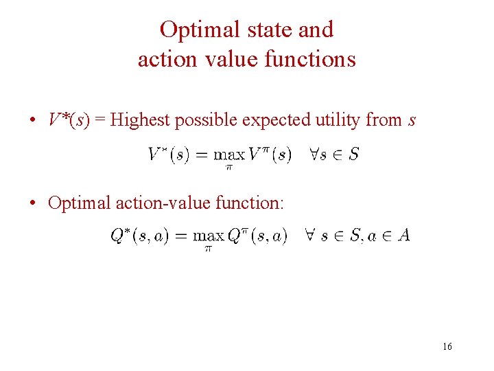
Optimal state and action value functions • V*(s) = Highest possible expected utility from s • Optimal action-value function: 16

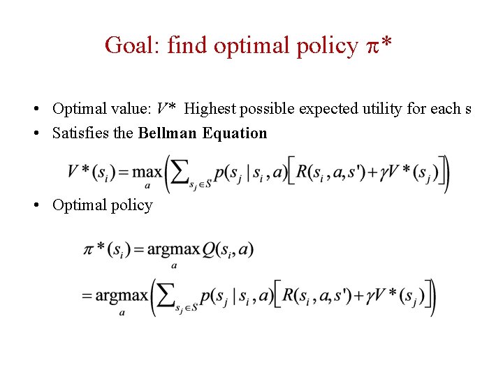
Goal: find optimal policy * • Optimal value: V* Highest possible expected utility for each s • Satisfies the Bellman Equation • Optimal policy

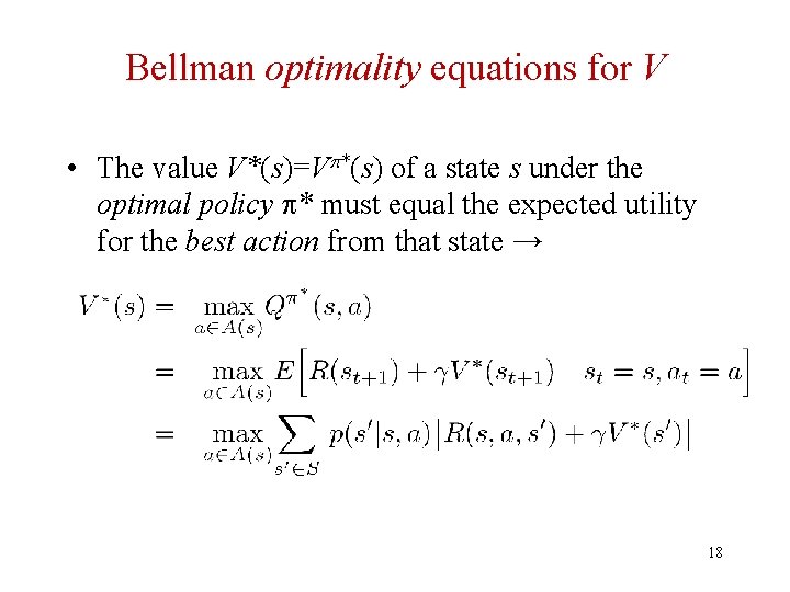
Bellman optimality equations for V • The value V*(s)=V *(s) of a state s under the optimal policy * must equal the expected utility for the best action from that state → 18

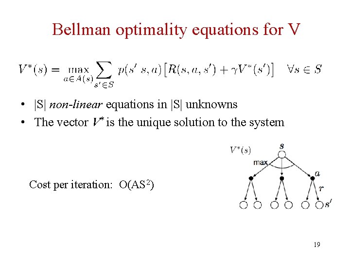
Bellman optimality equations for V • |S| non-linear equations in |S| unknowns • The vector V* is the unique solution to the system Cost per iteration: O(AS 2) 19

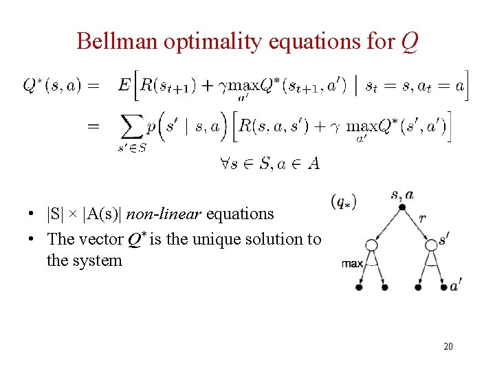
Bellman optimality equations for Q • |S| × |A(s)| non-linear equations • The vector Q* is the unique solution to the system 20

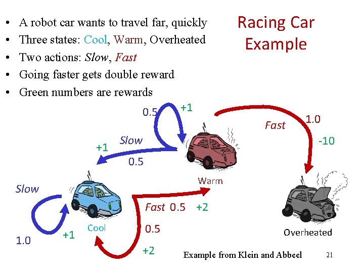
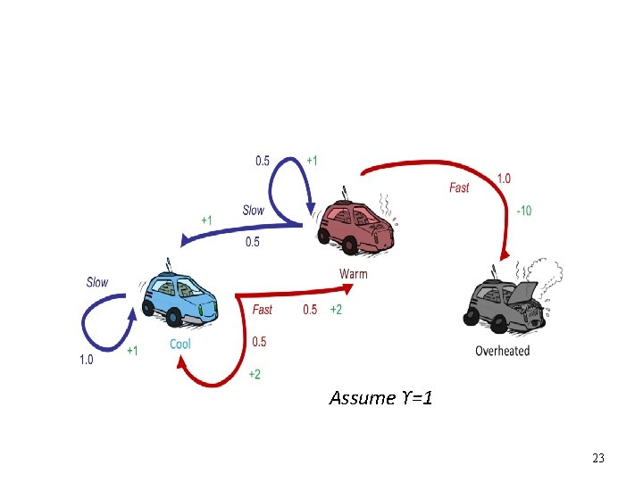
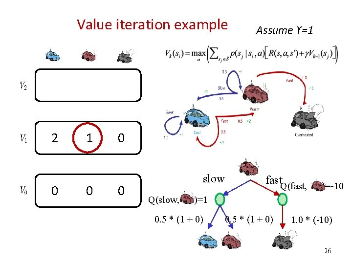
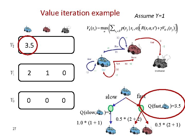
• • • A robot car wants to travel far, quickly Three states: Cool, Warm, Overheated Two actions: Slow, Fast Going faster gets double reward Green numbers are rewards +1 0. 5 +1 Racing Car Example Fast Slow 1. 0 -10 0. 5 Warm Slow Fast 0. 5 +2 1. 0 +1 Cool 0. 5 +2 Overheated Example from Klein and Abbeel 21

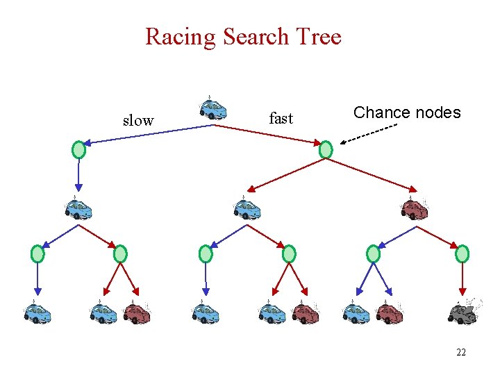
Racing Search Tree slow fast Chance nodes 22

Assume ϒ=1 Slide adapted from Klein and Abbeel 23

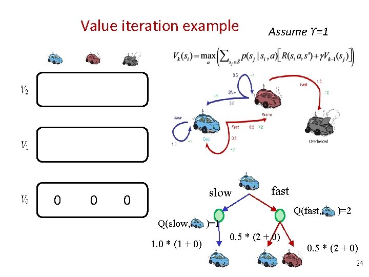
Value iteration example 0 0 slow 0 Assume ϒ=1 fast Q(fast, Q(slow, 1. 0 * (1 + 0) )=2 )=1 0. 5 * (2 + 0) Slide adapted from Klein and Abbeel 0. 5 * (2 + 0) 24

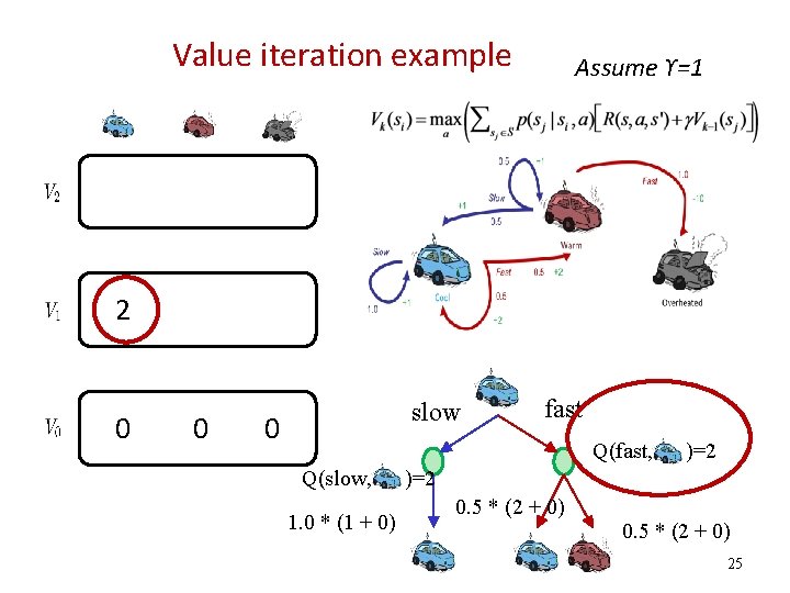
Value iteration example Assume ϒ=1 2 0 0 slow 0 fast Q(fast, Q(slow, 1. 0 * (1 + 0) )=2 0. 5 * (2 + 0) Slide adapted from Klein and Abbeel 0. 5 * (2 + 0) 25

Value iteration example 2 0 1 0 Assume ϒ=1 0 0 slow Q(slow, fast. Q(fast, )=-10 )=1 0. 5 * (1 + 0) 1. 0 * (-10) 26

Value iteration example Assume ϒ=1 3. 5 2 0 1 0 0 slow 0 Q(fast, Q(slow, 1. 0 * (1 + 1) 27 fast )=3. 5 )=2 0. 5 * (2 + 2) Slide adapted from Klein and Abbeel 0. 5 * (2 + 1)

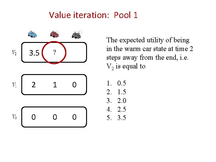
Value iteration: Pool 1 The expected utility of being in the warm car state at time 2 steps away from the end, i. e. V 2 is equal to 3. 5 ? 2 1 0 0 1. 2. 3. 4. 5. 0. 5 1. 5 2. 0 2. 5 3. 5

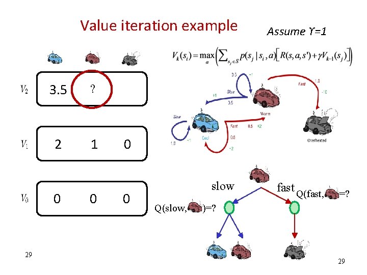
Value iteration example 3. 5 ? 2 1 0 29 0 Assume ϒ=1 0 0 slow Q(slow, fast Q(fast, =? )=? Slide adapted from Klein and Abbeel 29

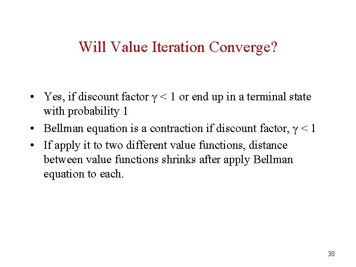
Will Value Iteration Converge? • Yes, if discount factor γ < 1 or end up in a terminal state with probability 1 • Bellman equation is a contraction if discount factor, γ < 1 • If apply it to two different value functions, distance between value functions shrinks after apply Bellman equation to each. 30

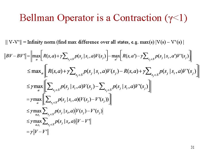
Bellman Operator is a Contraction (γ<1) || V-V’|| = Infinity norm (find max difference over all states, e. g. max(s) |V(s) – V’(s) | 31

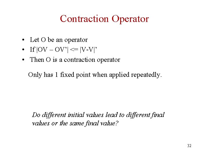
Contraction Operator • Let O be an operator • If |OV – OV’| <= |V-V|’ • Then O is a contraction operator Only has 1 fixed point when applied repeatedly. Do different initial values lead to different final values or the same final value? 32

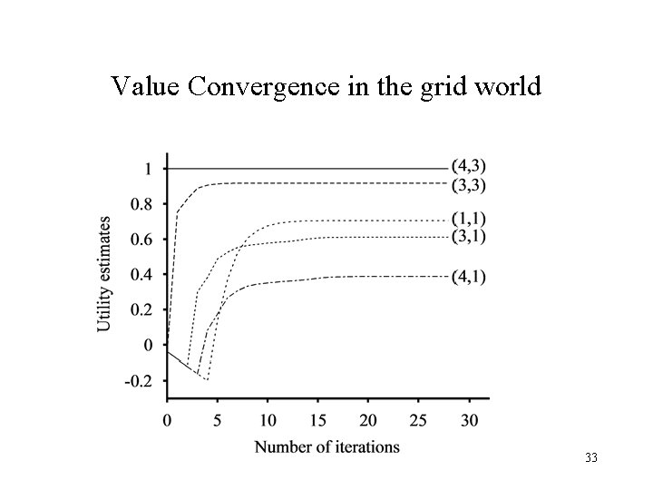
Value Convergence in the grid world 33

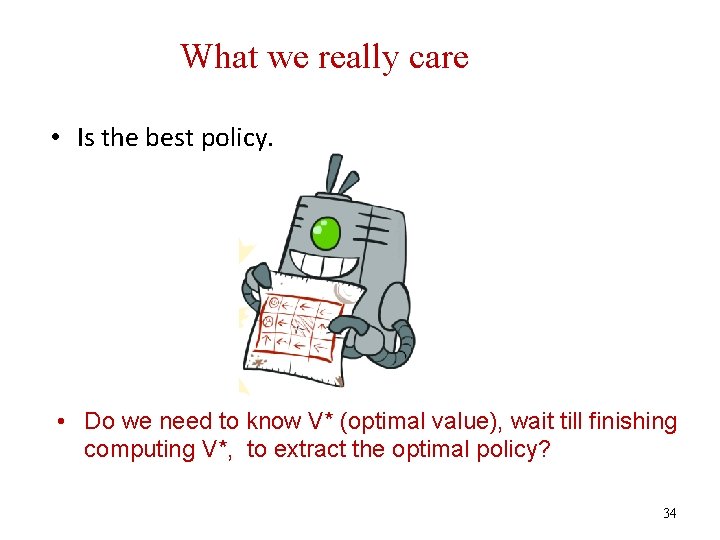
What we really care • Is the best policy. • Do we need to know V* (optimal value), wait till finishing computing V*, to extract the optimal policy? 34

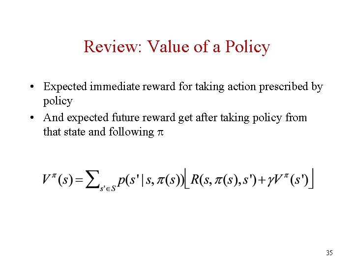
Review: Value of a Policy • Expected immediate reward for taking action prescribed by policy • And expected future reward get after taking policy from that state and following 35

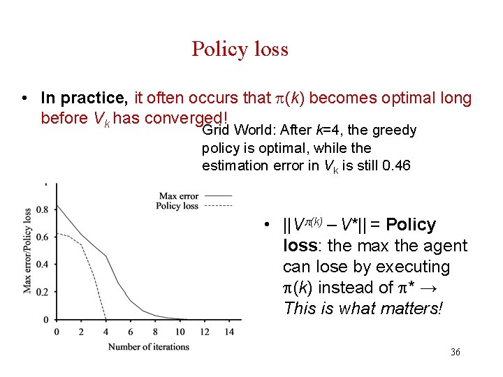
Policy loss • In practice, it often occurs that (k) becomes optimal long before Vk has converged! Grid World: After k=4, the greedy policy is optimal, while the estimation error in Vk is still 0. 46 • ||V (k) – V*|| = Policy loss: the max the agent can lose by executing (k) instead of * → This is what matters! 36

Finding optimal policy • If one action (the optimal) gets really better than the others, the exact magnitude of the V(s) doesn’t really matter to select the action in the greedy policy (i. e. , don’t need “precise” V values), more important are relative proportions. 37

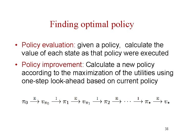
Finding optimal policy • Policy evaluation: given a policy, calculate the value of each state as that policy were executed • Policy improvement: Calculate a new policy according to the maximization of the utilities using one-step look-ahead based on current policy 38

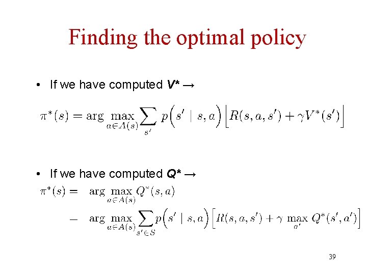
Finding the optimal policy • If we have computed V* → • If we have computed Q* → 39

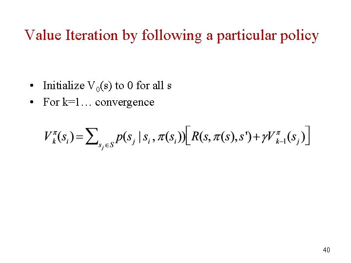
Value Iteration by following a particular policy • Initialize V 0(s) to 0 for all s • For k=1… convergence 40

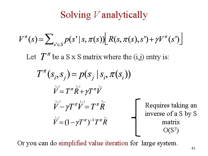
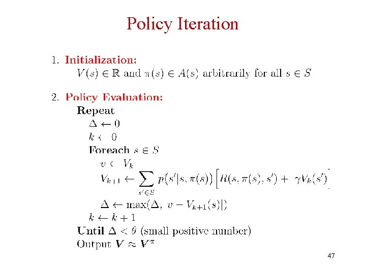
Solving V analytically Let be a S x S matrix where the (i, j) entry is: Requires taking an inverse of a S by S matrix O(S 3) Or you can do simplified value iteration for large system. 41

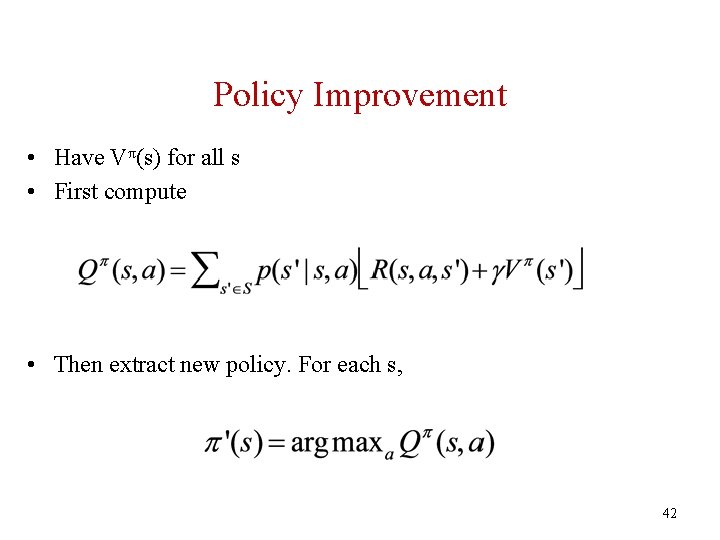
Policy Improvement • Have Vπ(s) for all s • First compute • Then extract new policy. For each s, 42

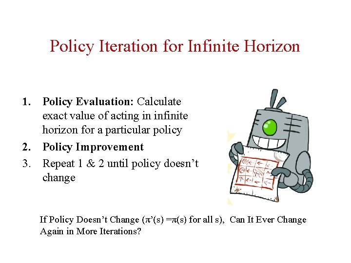
Policy Iteration for Infinite Horizon 1. Policy Evaluation: Calculate exact value of acting in infinite horizon for a particular policy 2. Policy Improvement 3. Repeat 1 & 2 until policy doesn’t change If Policy Doesn’t Change (π’(s) =π(s) for all s), Can It Ever Change Again in More Iterations?

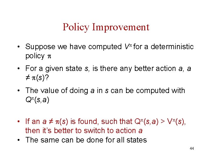
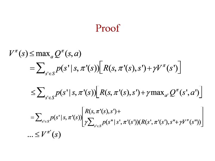
Policy Improvement • Suppose we have computed V for a deterministic policy • For a given state s, is there any better action a, a ≠ (s)? • The value of doing a in s can be computed with Q (s, a) • If an a ≠ (s) is found, such that Q (s, a) > V (s), then it’s better to switch to action a • The same can be done for all states 44

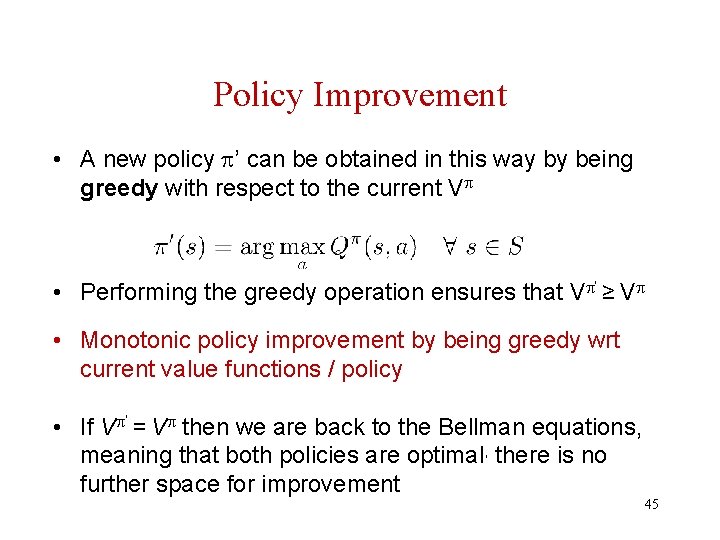
Policy Improvement • A new policy ’ can be obtained in this way by being greedy with respect to the current V • Performing the greedy operation ensures that V ’ ≥ V • Monotonic policy improvement by being greedy wrt current value functions / policy • If V ’ = V then we are back to the Bellman equations, meaning that both policies are optimal, there is no further space for improvement 45

Proof

Policy Iteration 47

Policy Iteration 48

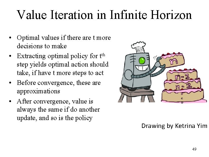
Value Iteration in Infinite Horizon • Optimal values if there are t more decisions to make • Extracting optimal policy for tth step yields optimal action should take, if have t more steps to act • Before convergence, these are approximations • After convergence, value is always the same if do another update, and so is the policy Drawing by Ketrina Yim 49

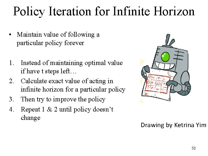
Policy Iteration for Infinite Horizon • Maintain value of following a particular policy forever 1. Instead of maintaining optimal value if have t steps left… 2. Calculate exact value of acting in infinite horizon for a particular policy 3. Then try to improve the policy 4. Repeat 1 & 2 until policy doesn’t change Drawing by Ketrina Yim 50

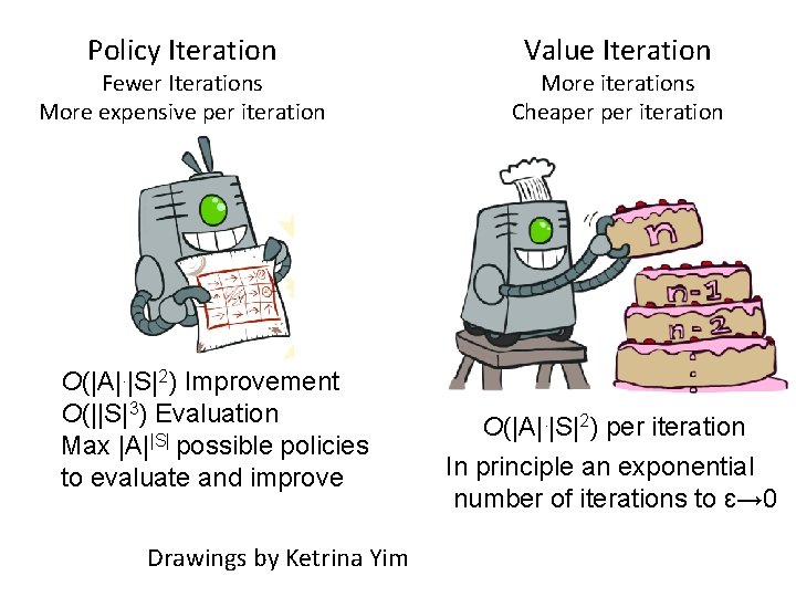
Policy Iteration Fewer Iterations More expensive per iteration O(|A|. |S|2) Improvement O(||S|3) Evaluation Max |A||S| possible policies to evaluate and improve Drawings by Ketrina Yim Value Iteration More iterations Cheaper iteration O(|A|. |S|2) per iteration In principle an exponential number of iterations to ɛ→ 0

MDPs: What You Should Know • Definition • How to define for a problem • Value iteration and policy iteration – How to implement – Convergence guarantees – Computational complexity