Markov Chains Summary n n Markov Chains Discrete

- Slides: 55

Markov Chains

Summary n n Markov Chains Discrete Time Markov Chains ¨ Homogeneous and non-homogeneous Markov chains ¨ Transient and steady state Markov chains n Continuous Time Markov Chains ¨ Homogeneous and non-homogeneous Markov chains ¨ Transient and steady state Markov chains

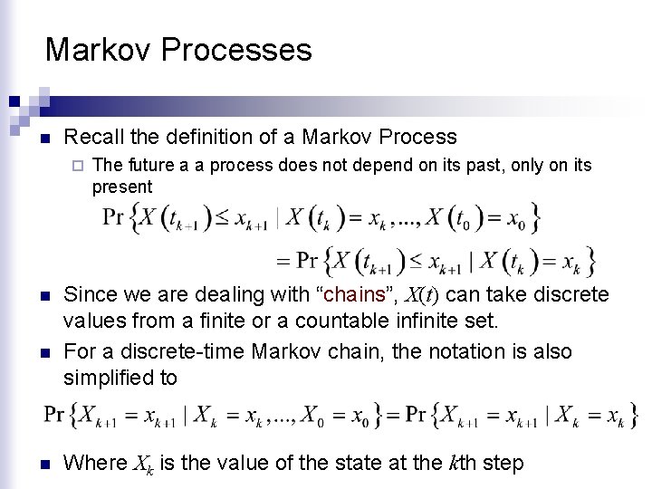
Markov Processes n Recall the definition of a Markov Process ¨ n n n The future a a process does not depend on its past, only on its present Since we are dealing with “chains”, X(t) can take discrete values from a finite or a countable infinite set. For a discrete-time Markov chain, the notation is also simplified to Where Xk is the value of the state at the kth step

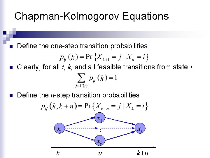
Chapman-Kolmogorov Equations n Define the one-step transition probabilities n Clearly, for all i, k, and all feasible transitions from state i n Define the n-step transition probabilities x 1 … xi xj x. R k u k+n

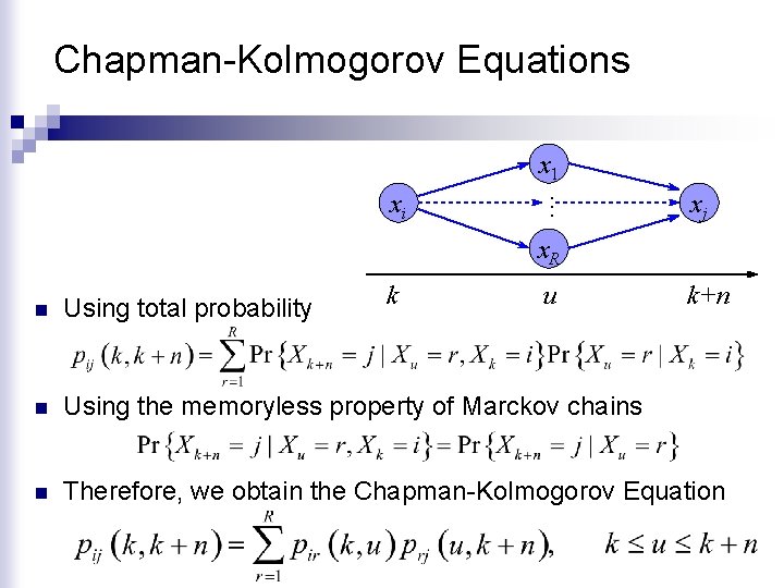
Chapman-Kolmogorov Equations x 1 … xi xj x. R k u k+n n Using total probability n Using the memoryless property of Marckov chains n Therefore, we obtain the Chapman-Kolmogorov Equation

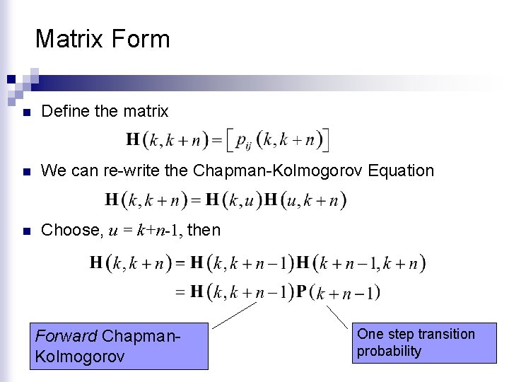
Matrix Form n Define the matrix n We can re-write the Chapman-Kolmogorov Equation n Choose, u = k+n-1, then Forward Chapman. Kolmogorov One step transition probability

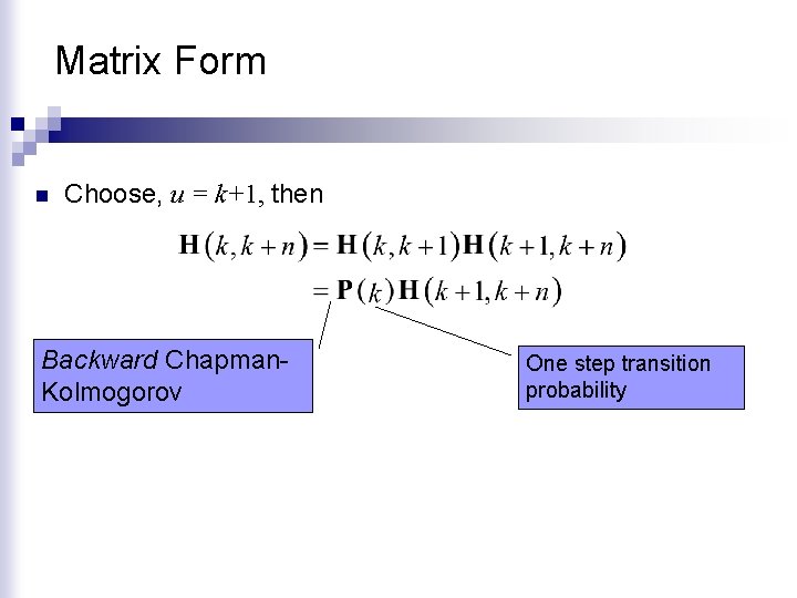
Matrix Form n Choose, u = k+1, then Backward Chapman. Kolmogorov One step transition probability

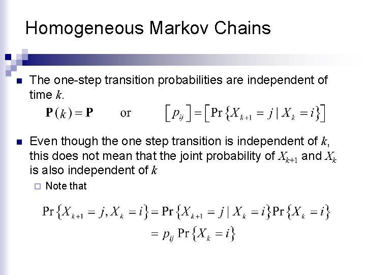
Homogeneous Markov Chains n The one-step transition probabilities are independent of time k. n Even though the one step transition is independent of k, this does not mean that the joint probability of Xk+1 and Xk is also independent of k ¨ Note that

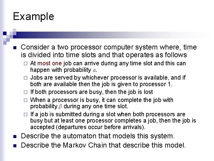
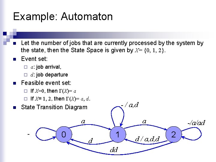
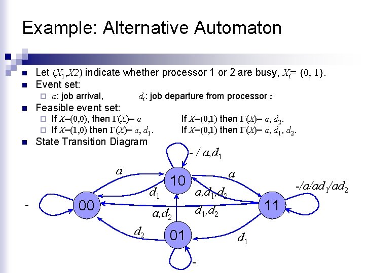
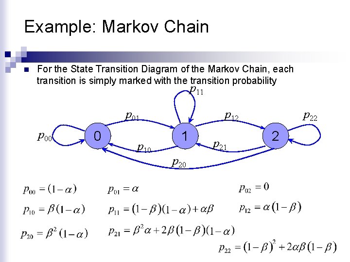
Example n Consider a two processor computer system where, time is divided into time slots and that operates as follows ¨ ¨ ¨ n n At most one job can arrive during any time slot and this can happen with probability α. Jobs are served by whichever processor is available, and if both are available then the job is given to processor 1. If both processors are busy, then the job is lost When a processor is busy, it can complete the job with probability β during any one time slot. If a job is submitted during a slot when both processors are busy but at least one processor completes a job, then the job is accepted (departures occur before arrivals). Describe the automaton that models this system. Describe the Markov Chain that describe this model.

Example: Automaton n n Let the number of jobs that are currently processed by the system by the state, then the State Space is given by X= {0, 1, 2}. Event set: a: job arrival, ¨ d: job departure ¨ n Feasible event set: If X=0, then Γ(X)= a ¨ If X= 1, 2, then Γ(Χ)= a, d. ¨ n - / a, d State Transition Diagram a - 0 a d 1 dd d / a, d, d -/a/ad 2

Example: Alternative Automaton n n Let (X 1, X 2) indicate whether processor 1 or 2 are busy, Xi= {0, 1}. Event set: ¨ n Feasible event set: ¨ ¨ n a: job arrival, di: job departure from processor i If X=(0, 0), then Γ(X)= a If X=(1, 0) then Γ(Χ)= a, d 1. State Transition Diagram - / a, d 1 a - If X=(0, 1) then Γ(Χ)= a, d 2. If X=(0, 1) then Γ(Χ)= a, d 1, d 2. d 1 00 10 a, d 2 a -/a/ad 1/ad 2 a, d 1, d 2 01 11 d 1 -

Example: Markov Chain n For the State Transition Diagram of the Markov Chain, each transition is simply marked with the transition probability p 11 p 00 0 p 12 1 p 20 p 21 p 22 2

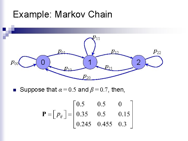
Example: Markov Chain p 11 p 00 n 0 p 12 1 p 20 Suppose that α = 0. 5 and β = 0. 7, then, p 22 2

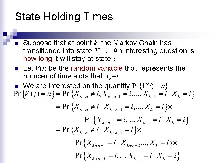
State Holding Times n n n Suppose that at point k, the Markov Chain has transitioned into state Xk=i. An interesting question is how long it will stay at state i. Let V(i) be the random variable that represents the number of time slots that Xk=i. We are interested on the quantity Pr{V(i) = n}

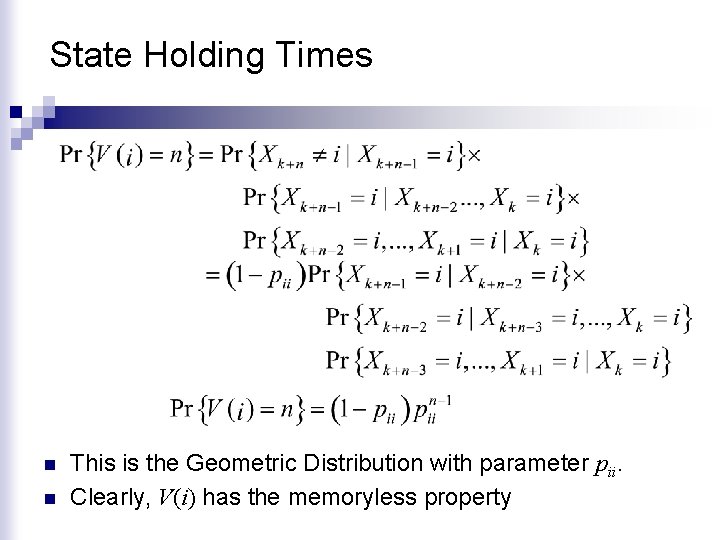
State Holding Times n n This is the Geometric Distribution with parameter pii. Clearly, V(i) has the memoryless property

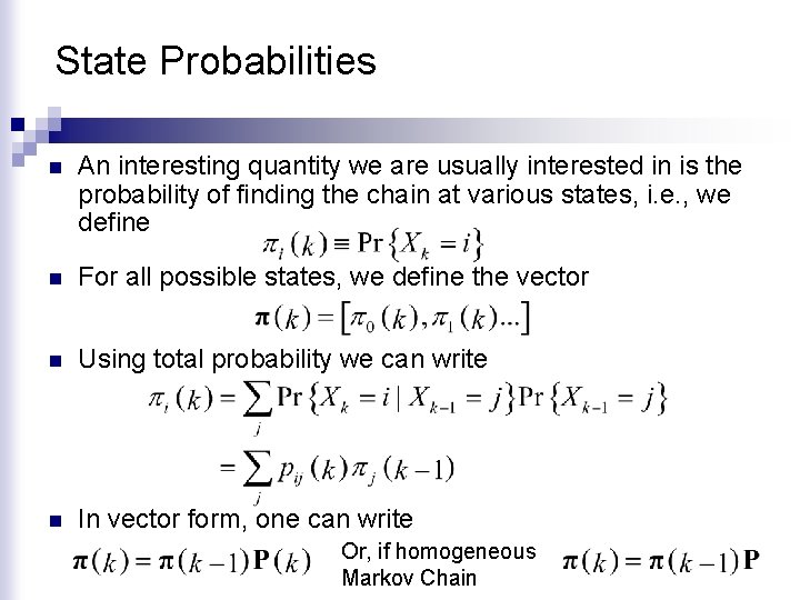
State Probabilities n An interesting quantity we are usually interested in is the probability of finding the chain at various states, i. e. , we define n For all possible states, we define the vector n Using total probability we can write n In vector form, one can write Or, if homogeneous Markov Chain

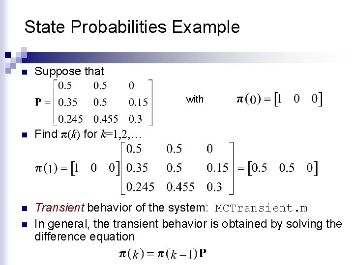
State Probabilities Example n Suppose that with n Find π(k) for k=1, 2, … n Transient behavior of the system: MCTransient. m In general, the transient behavior is obtained by solving the difference equation n

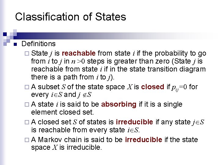
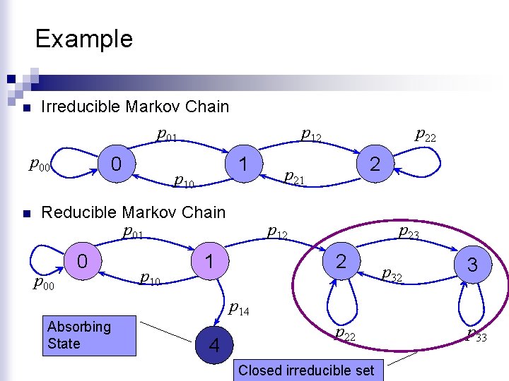
Classification of States n Definitions ¨ State j is reachable from state i if the probability to go from i to j in n >0 steps is greater than zero (State j is reachable from state i if in the state transition diagram there is a path from i to j). ¨ A subset S of the state space X is closed if pij=0 for every i S and j S ¨ A state i is said to be absorbing if it is a single element closed set. ¨ A closed set S of states is irreducible if any state j S is reachable from every state i S. ¨ A Markov chain is said to be irreducible if the state space X is irreducible.

Example n Irreducible Markov Chain p 01 p 00 n 0 p 12 1 p 10 Reducible Markov Chain p 01 p 00 0 p 10 p 22 2 p 21 p 12 1 p 23 2 p 32 3 p 14 Absorbing State 4 p 22 Closed irreducible set p 33

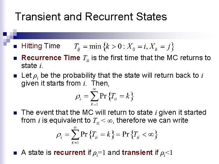
Transient and Recurrent States n Hitting Time n Recurrence Time Tii is the first time that the MC returns to state i. Let ρi be the probability that the state will return back to i given it starts from i. Then, n n The event that the MC will return to state i given it started from i is equivalent to Tii < ∞, therefore we can write n A state is recurrent if ρi=1 and transient if ρi<1

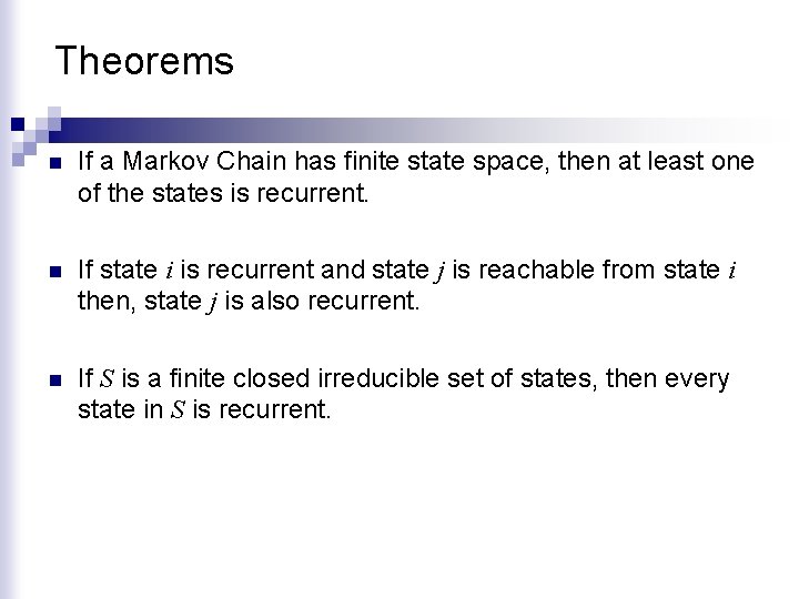
Theorems n If a Markov Chain has finite state space, then at least one of the states is recurrent. n If state i is recurrent and state j is reachable from state i then, state j is also recurrent. n If S is a finite closed irreducible set of states, then every state in S is recurrent.

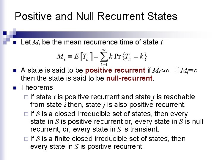
Positive and Null Recurrent States n Let Mi be the mean recurrence time of state i n A state is said to be positive recurrent if Mi<∞. If Mi=∞ then the state is said to be null-recurrent. Theorems ¨ If state i is positive recurrent and state j is reachable from state i then, state j is also positive recurrent. ¨ If S is a closed irreducible set of states, then every state in S is positive recurrent or, every state in S is null recurrent, or, every state in S is transient. ¨ If S is a finite closed irreducible set of states, then every state in S is positive recurrent. n

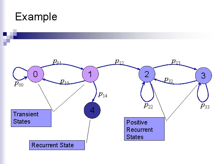
Example p 01 p 00 0 p 12 1 p 23 2 p 32 3 p 14 Transient States Recurrent State 4 p 22 Positive Recurrent States p 33

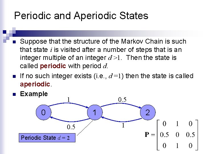
Periodic and Aperiodic States n n n Suppose that the structure of the Markov Chain is such that state i is visited after a number of steps that is an integer multiple of an integer d >1. Then the state is called periodic with period d. If no such integer exists (i. e. , d =1) then the state is called aperiodic. Example 1 0. 5 0 1 0. 5 Periodic State d = 2 2 1

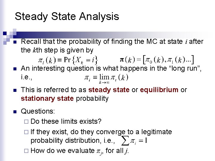
Steady State Analysis n Recall that the probability of finding the MC at state i after the kth step is given by n An interesting question is what happens in the “long run”, i. e. , n This is referred to as steady state or equilibrium or stationary state probability n Questions: ¨ Do these limits exists? ¨ If they exist, do they converge to a legitimate probability distribution, i. e. , ¨ How do we evaluate πj, for all j.

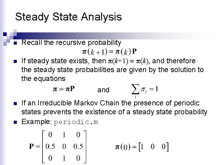
Steady State Analysis n Recall the recursive probability n If steady state exists, then π(k+1) π(k), and therefore the steady state probabilities are given by the solution to the equations and n n If an Irreducible Markov Chain the presence of periodic states prevents the existence of a steady state probability Example: periodic. m

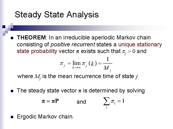
Steady State Analysis n THEOREM: In an irreducible aperiodic Markov chain consisting of positive recurrent states a unique stationary state probability vector π exists such that πj > 0 and where Mj is the mean recurrence time of state j n The steady state vector π is determined by solving and n Ergodic Markov chain.

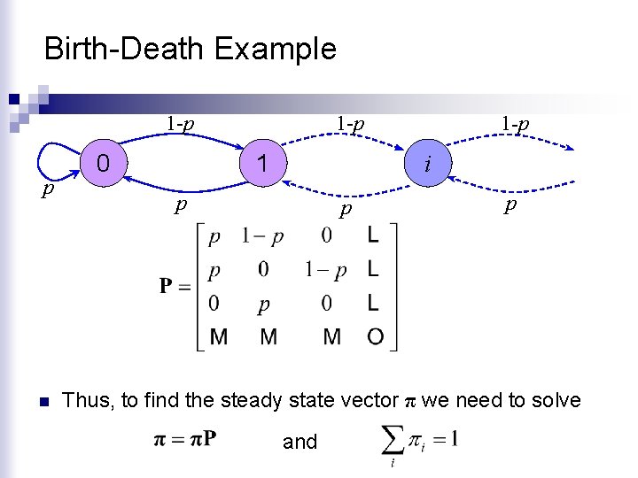
Birth-Death Example 1 -p p n 0 1 -p 1 1 -p i p p p Thus, to find the steady state vector π we need to solve and

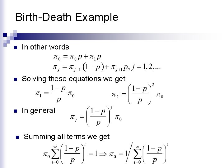
Birth-Death Example n In other words n Solving these equations we get n In general n Summing all terms we get

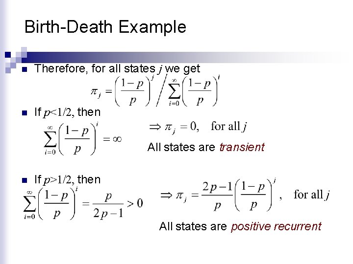
Birth-Death Example n Therefore, for all states j we get n If p<1/2, then All states are transient n If p>1/2, then All states are positive recurrent

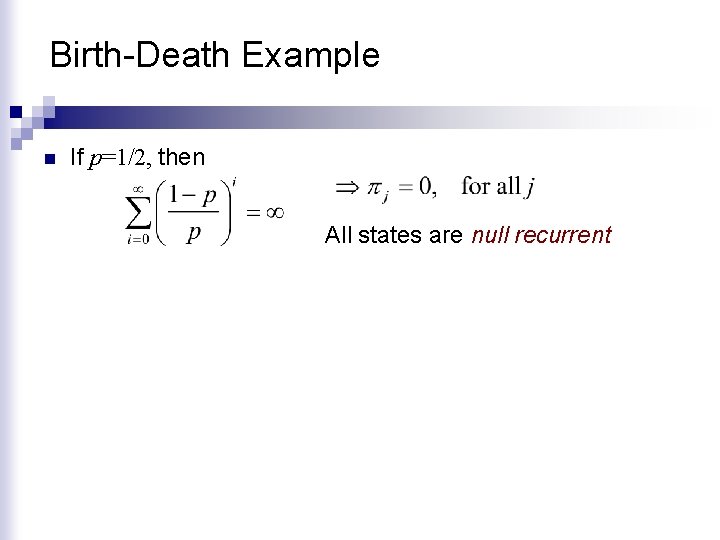
Birth-Death Example n If p=1/2, then All states are null recurrent

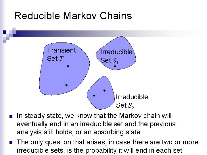
Reducible Markov Chains Transient Set T Irreducible Set S 1 Irreducible Set S 2 n n In steady state, we know that the Markov chain will eventually end in an irreducible set and the previous analysis still holds, or an absorbing state. The only question that arises, in case there are two or more irreducible sets, is the probability it will end in each set

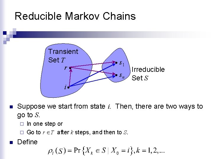
Reducible Markov Chains Transient Set T r s 1 sn Irreducible Set S i n Suppose we start from state i. Then, there are two ways to go to S. In one step or ¨ Go to r T after k steps, and then to S. ¨ n Define

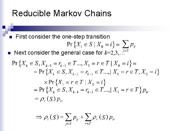
Reducible Markov Chains n n First consider the one-step transition Next consider the general case for k=2, 3, …

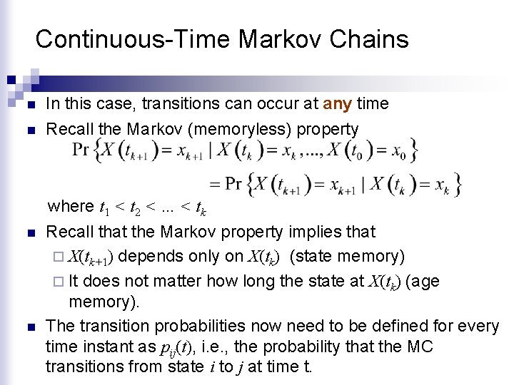
Continuous-Time Markov Chains n n In this case, transitions can occur at any time Recall the Markov (memoryless) property where t 1 < t 2 < … < tk n n Recall that the Markov property implies that ¨ X(tk+1) depends only on X(tk) (state memory) ¨ It does not matter how long the state at X(tk) (age memory). The transition probabilities now need to be defined for every time instant as pij(t), i. e. , the probability that the MC transitions from state i to j at time t.

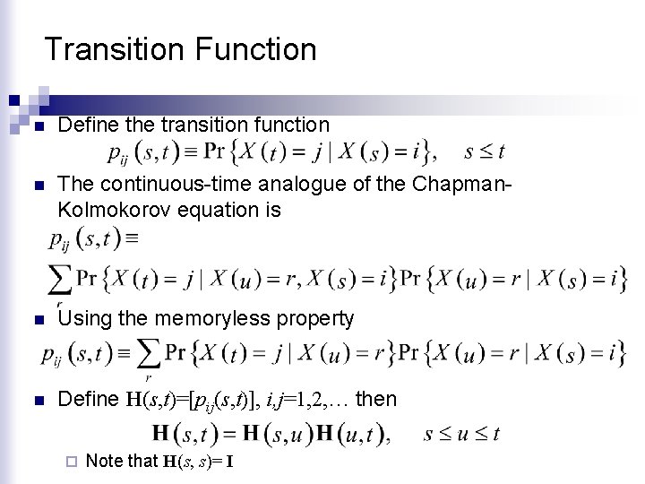
Transition Function n Define the transition function n The continuous-time analogue of the Chapman. Kolmokorov equation is n Using the memoryless property n Define H(s, t)=[pij(s, t)], i, j=1, 2, … then ¨ Note that H(s, s)= I

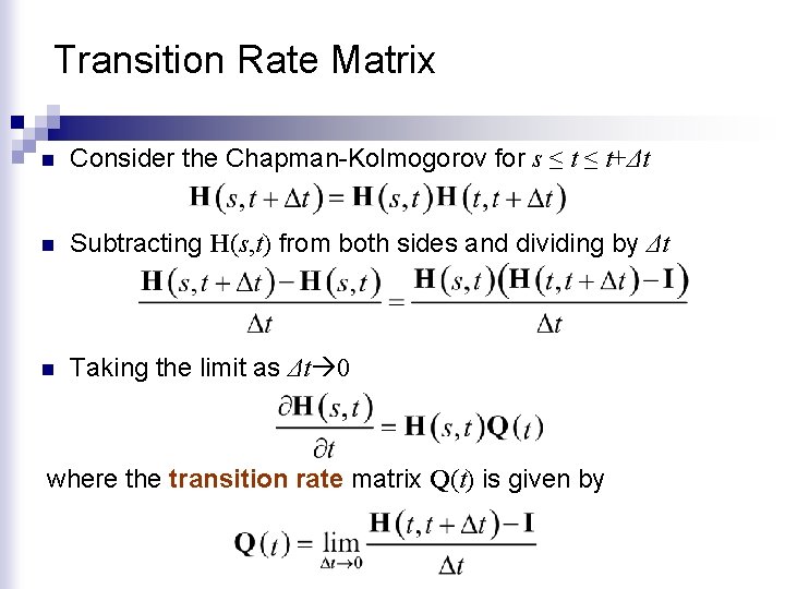
Transition Rate Matrix n Consider the Chapman-Kolmogorov for s ≤ t+Δt n Subtracting H(s, t) from both sides and dividing by Δt n Taking the limit as Δt 0 where the transition rate matrix Q(t) is given by

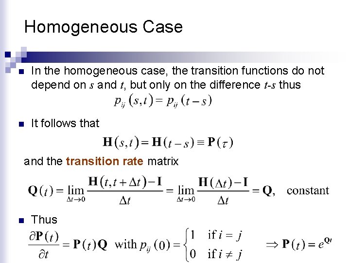
Homogeneous Case n In the homogeneous case, the transition functions do not depend on s and t, but only on the difference t-s thus n It follows that and the transition rate matrix n Thus

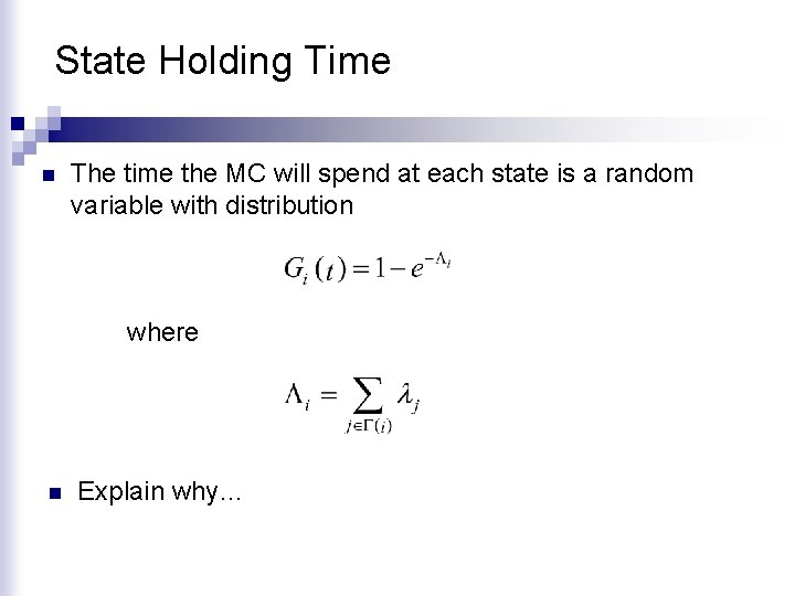
State Holding Time n The time the MC will spend at each state is a random variable with distribution where n Explain why…

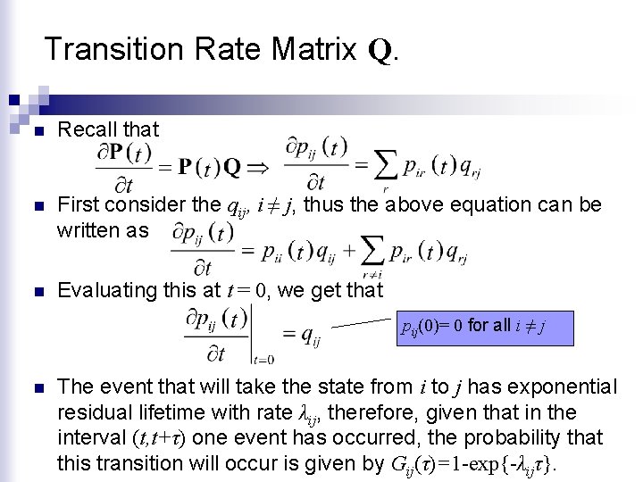
Transition Rate Matrix Q. n Recall that n First consider the qij, i ≠ j, thus the above equation can be written as n Evaluating this at t = 0, we get that pij(0)= 0 for all i ≠ j n The event that will take the state from i to j has exponential residual lifetime with rate λij, therefore, given that in the interval (t, t+τ) one event has occurred, the probability that this transition will occur is given by Gij(τ)=1 -exp{-λijτ}.

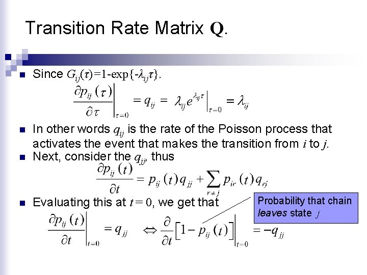
Transition Rate Matrix Q. n Since Gij(τ)=1 -exp{-λijτ}. n n In other words qij is the rate of the Poisson process that activates the event that makes the transition from i to j. Next, consider the qjj, thus n Evaluating this at t = 0, we get that Probability that chain leaves state j

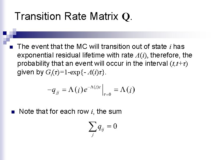
Transition Rate Matrix Q. n n The event that the MC will transition out of state i has exponential residual lifetime with rate Λ(i), therefore, the probability that an event will occur in the interval (t, t+τ) given by Gi(τ)=1 -exp{- Λ(i)τ}. Note that for each row i, the sum

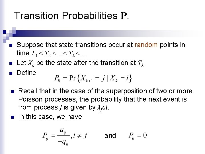
Transition Probabilities P. n n n Suppose that state transitions occur at random points in time T 1 < T 2 <…< Tk <… Let Xk be the state after the transition at Tk Define Recall that in the case of the superposition of two or more Poisson processes, the probability that the next event is from process j is given by λj/Λ. In this case, we have and

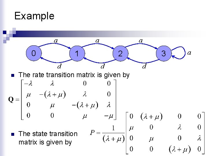
Example n n n n Assume a computer system where jobs arrive according to a Poisson process with rate λ. Each job is processed using a First In First Out (FIFO) policy. The processing time of each job is exponential with rate μ. The computer has buffer to store up to two jobs that wait for processing. Jobs that find the buffer full are lost. Draw the state transition diagram. Find the Rate Transition Matrix Q. Find the State Transition Matrix P

Example a 0 n n a 1 a 2 d d The rate transition matrix is given by The state transition matrix is given by 3 d a

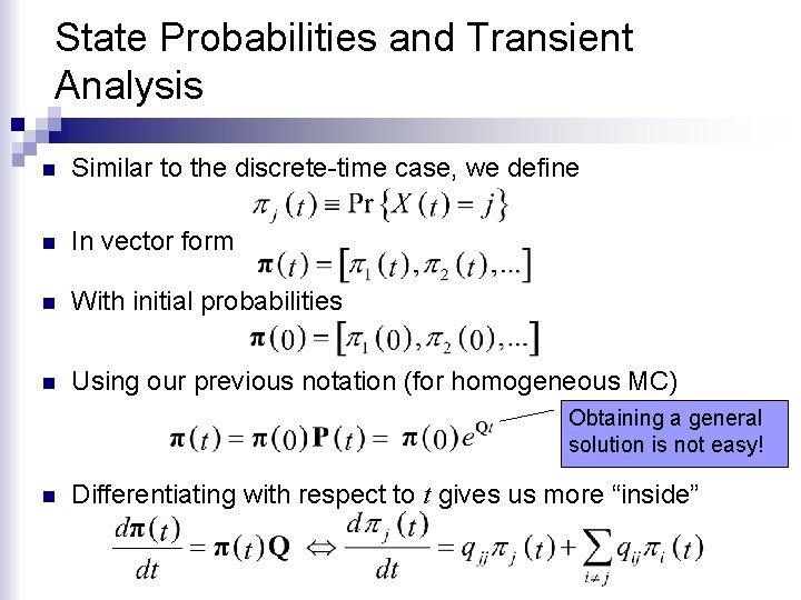
State Probabilities and Transient Analysis n Similar to the discrete-time case, we define n In vector form n With initial probabilities n Using our previous notation (for homogeneous MC) Obtaining a general solution is not easy! n Differentiating with respect to t gives us more “inside”

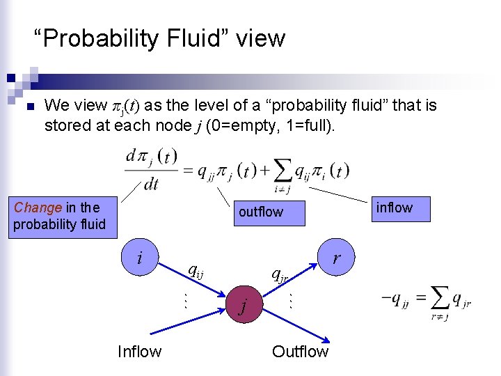
“Probability Fluid” view n We view πj(t) as the level of a “probability fluid” that is stored at each node j (0=empty, 1=full). Change in the probability fluid inflow outflow i qij j … … Inflow qjr Outflow r

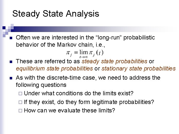
Steady State Analysis n Often we are interested in the “long-run” probabilistic behavior of the Markov chain, i. e. , n These are referred to as steady state probabilities or equilibrium state probabilities or stationary state probabilities n As with the discrete-time case, we need to address the following questions ¨ Under what conditions do the limits exist? ¨ If they exist, do they form legitimate probabilities? ¨ How can we evaluate these limits?

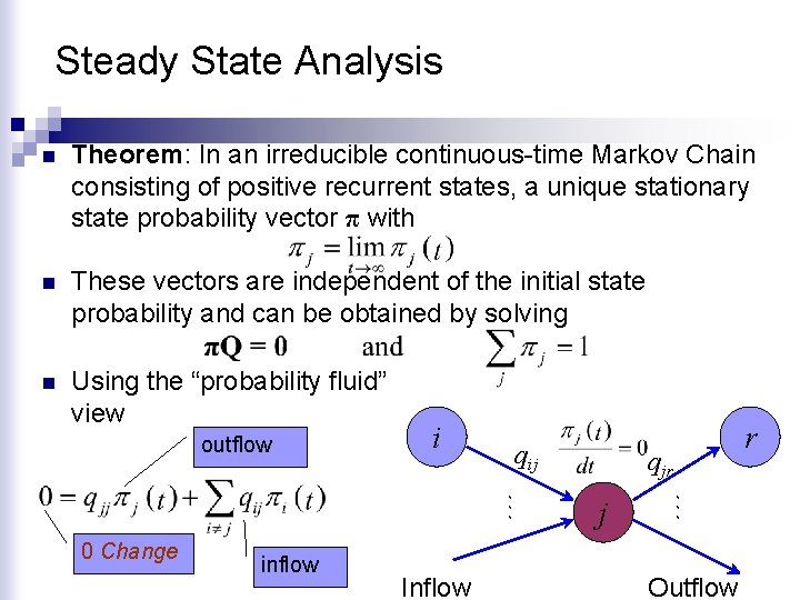
Steady State Analysis n Theorem: In an irreducible continuous-time Markov Chain consisting of positive recurrent states, a unique stationary state probability vector π with n These vectors are independent of the initial state probability and can be obtained by solving n Using the “probability fluid” view outflow i qij inflow Inflow j … … 0 Change qjr Outflow r

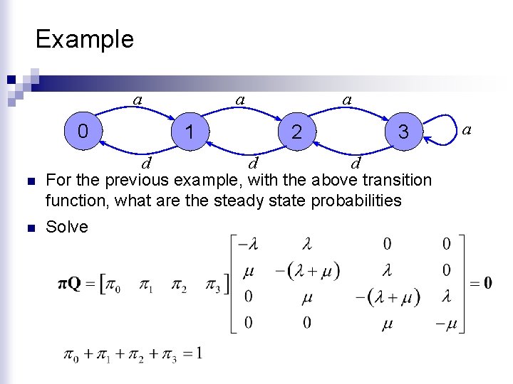
Example a 0 a 1 a 2 3 n d d d For the previous example, with the above transition function, what are the steady state probabilities n Solve a

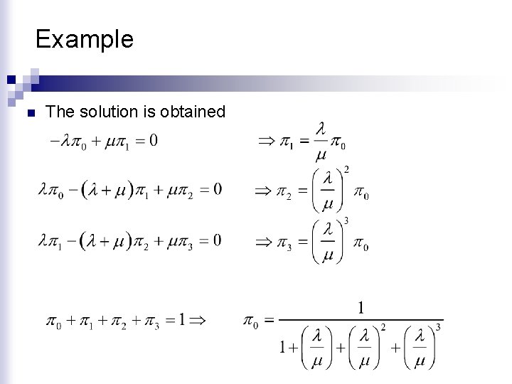
Example n The solution is obtained

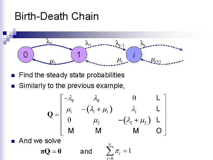
Birth-Death Chain λ 0 0 μ 1 λ 1 1 λi-1 μi n Find the steady state probabilities Similarly to the previous example, n And we solve n and λi i μi+1

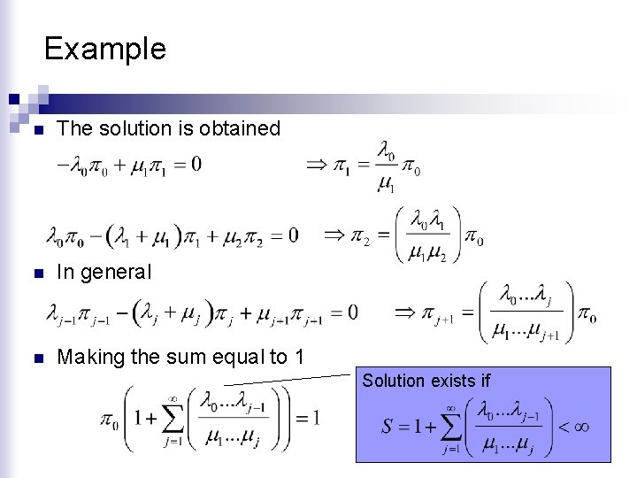
Example n The solution is obtained n In general n Making the sum equal to 1 Solution exists if

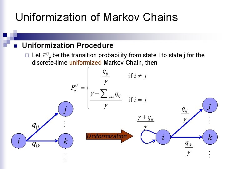
Uniformization of Markov Chains n n n In general, discrete-time models are easier to work with, and computers (that are needed to solve such models) operate in discrete-time Thus, we need a way to turn continuous-time to discretetime Markov Chains Uniformization Procedure ¨ Recall that the total rate out of state i is –qii=Λ(i). Pick a uniform rate γ such that γ ≥ Λ(i) for all states i. ¨ The difference γ - Λ(i) implies a “fictitious” event that returns the MC back to state i (self loop).

Uniformization of Markov Chains n Uniformization Procedure ¨ Let PUij be the transition probability from state I to state j for the discrete-time uniformized Markov Chain, then j j qik … i … qij k Uniformization i k … …