Rock suites trace elements and radiogenic isotopes GEOS

Rock suites, trace elements and radiogenic isotopes GEOS 408/508 Lectures 4 -6

l Mg. O and Fe. O l Al 2 O 3 and Ca. O l Si. O 2 l Na 2 O, K 2 O, Ti. O 2, P 2 O 5

Rock suites l l The totality of major compositions found in a spatio-temporal domain of interest; Typically display a range of major, trace and isotopic compositions; Examples: calc-alkaline (banatite) suites in arc regions; bimodal (basalt -rhyolite) suites in continental extension, etc; Perhaps the most important lesson to take home regarding rocks suites is that no single magmatic rock composition can be indicative of a past tectonic setting - use instead the range of rock compositions.

More Trace Elements Note magnitue of major element changes Harker variation diagram for 310 analyzed volcanic rocks from Crater Lake (Mt. Mazama), Oregon Cascades. Data compiled by Rick Conrey (personal communication). From Winter (2001) An Introduction to Igneous and Metamorphic Petrology. Prentice Hall.

Generating diversity l l l Fractionation = selective crystallization and removal of crystals from an evolving magma; Mixing= co-aggregation of two (or more) different magmas; Unmixxing (not common) = Generation of two liquids out of one via melt immiscibility; Assimilation and fractional crystallization (AFC)= wall rock incorporation coupled with internal fractionation; Source heterogeneity; “secondary”, postmagmatic processes = hydrothermal alteration, weathering, etc.

Bivariate (x-y) diagrams Harker diagram for Crater Lake Figure 2. Harker variation diagram for 310 analyzed volcanic rocks from Crater Lake (Mt. Mazama), Oregon Cascades. Data compiled by Rick Conrey (personal communication).

Bivariate (x-y) diagrams Harker diagram for Crater Lake Figure 2. Harker variation diagram for 310 analyzed volcanic rocks from Crater Lake (Mt. Mazama), Oregon Cascades. Data compiled by Rick Conrey (personal communication).

Models of Magmatic Evolution Table 5. Chemical analyses (wt. %) of a hypothetical set of related volcanics. Oxide Si. O 2 Ti. O 2 Al 2 O 3 Fe 2 O 3* Mg. O Ca. O Na 2 O K 2 O B 50. 2 1. 1 14. 9 10. 4 7. 4 10. 0 2. 6 1. 0 BA 54. 3 0. 8 15. 7 9. 2 3. 7 8. 2 3. 2 2. 1 A 60. 1 0. 7 16. 1 6. 9 2. 8 5. 9 3. 8 2. 5 D 64. 9 0. 6 16. 4 5. 1 1. 7 3. 6 2. 5 RD 66. 2 0. 5 15. 3 5. 1 0. 9 3. 5 3. 9 3. 1 R 71. 5 0. 3 14. 1 2. 8 0. 5 1. 1 3. 4 4. 1 LOI Total 1. 9 99. 5 2. 0 1. 8 1. 6 99. 2 100. 6 100. 0 1. 2 99. 7 1. 4 99. 2 B = basalt, BA = basaltic andesite, A = andesite, D = dacite, RD = rhyo-dacite, R = rhyolite. Data from Ragland (1989)

Harker diagram Smooth trends F Model with 3 assumptions: 1 Rocks are related by FX 2 Trends = liquid line of descent 3 The basalt is the parent magma from which the others are derived F Figure 7. Stacked variation diagrams of hypothetical components X and Y (either weight or mol %). P = parent, D = daughter, S = solid extract, A, B, C = possible extracted solid phases. For explanation, see text. From Ragland (1989). Basic Analytical Petrology, Oxford Univ. Press.

l l Extrapolate BA B and further to low Si. O 2 K 2 O is first element to 0 (at Si. O 2 = 46. 5) 46. 5% Si. O 2 is interpreted to be the concentration in the bulk solid extract and the blue line the concentration of all other oxides Figure 7. Stacked Harker diagrams for the calc-alkaline volcanic series of Table 8 -5 (dark circles). From Ragland (1989). Basic Analytical Petrology, Oxford Univ. Press.

Extrapolate the other curves back BA B blue line and read off X of mineral extract Results: Remove plagioclase, olivine, pyroxene and Fe-Ti oxide Oxide Wt% Cation Norm Si. O 2 Ti. O 2 Al 2 O 3 Fe 2 O 3* Mg. O Ca. O Na 2 O K 2 O Total 46. 5 1. 4 14. 2 11. 5 10. 8 11. 5 2. 1 0 98. 1 ab an di hy ol mt il 18. 3 30. 1 23. 2 4. 7 19. 3 1. 7 2. 7 100 Then repeat for each increment BA A etc.

Now note magnitude of trace element changes Figure 1. Harker Diagram for Crater Lake. From data compiled by Rick Conrey. From Winter (2001) An Introduction to Igneous and Metamorphic Petrology. Prentice Hall.

Element Distribution Goldschmidt’s rules (simplistic, but useful) 1. 2 ions with the same valence and radius should exchange easily and enter a solid solution in amounts equal to their overall proportions

Goldschmidt’s rules 2. If 2 ions have a similar radius and the same valence: the smaller ion is preferentially incorporated into the solid over the liquid

3. If 2 ions have a similar radius, but different valence: the ion with the higher charge is preferentially incorporated into the solid over the liquid

Chemical Fractionation l The uneven distribution of an ion between two competing (equilibrium) phases

Exchange equilibrium of a component i between two phases (solid and liquid) i (liquid) = i (solid) eq. 2 K = a isolid liquid a i= K = equilibrium constant X solid i Xi liquid i

l l Trace element concentrations are in the Henry’s Law region of concentration, so their activity varies in direct relation to their concentration in the system Thus if XNi in the system doubles the XNi in all phases will double F This does not mean that XNi in all phases is the same, since trace elements do fractionate. Rather the XNi within each phase will vary in proportion to the system concentration

l incompatible elements are concentrated in the melt (KD or D) « 1 l compatible elements are concentrated in the solid KD or D » 1

l For dilute solutions can substitute D for KD: CS D= CL Where CS = the concentration of some element in the solid phase

l Incompatible elements commonly two subgroups Smaller, highly charged high field strength (HFS) elements (REE, Th, U, Ce, Pb 4+, Zr, Hf, Ti, Nb, Ta) F Low field strength large ion lithophile (LIL) elements (K, Rb, Cs, Ba, Pb 2+, Sr, Eu 2+) are mobile, particularly if a fluid phase is involved F

Compatibility depends on minerals and melts involved. Which are incompatible? Why?

l For a rock, determine the bulk distribution coefficient D for an element by calculating the contribution for each mineral eq. 4: Di = W A Di A WA = weight % of mineral A in the rock Di = partition coefficient of element i in A mineral A

Example: hypothetical garnet lherzolite = 60% olivine, 25% orthopyroxene, 10% clinopyroxene, and 5% garnet (all by weight), using the data in Table 9 -1, is: DEr = (0. 6 · 0. 026) + (0. 25 · 0. 23) + (0. 10 · 0. 583) + (0. 05 · 4. 7) = 0. 366

Homework 3 l Calculate partition coefficient of Sr for one (any) one of the rocks in Cecil’s data, assuming that the actual minerals are the norms you calculated for that rock. Get the Kd’s from GERM’s tabulated source online and use mineral-silicic melt coefficient.

l l Trace elements strongly partitioned into a single mineral Ni - olivine = 14 Figure 1 a. Ni Harker Diagram for Crater Lake. From data compiled by Rick Conrey. From Winter (2001) An Introduction to Igneous and Metamorphic Petrology. Prentice Hall.

l l Incompatible trace elements concentrate liquid Reflect the proportion of liquid at a given state of crystallization or melting Figure 1 b. Zr Harker Diagram for Crater Lake. From data compiled by Rick Conrey. From Winter (2001) An Introduction to Igneous and Metamorphic Petrology. Prentice Hall.

Trace element concentrations are in the Henry’s Law region of concentration, so their activity varies in direct relation to their concentration in the system

Trace element concentrations are in the Henry’s Law region of concentration, so their activity varies in direct relation to their concentration in the system Because of this, the ratios of trace elements are often superior to the concentration of a single element in identifying the role of a specific mineral

l K/Rb often used the importance of amphibole in a source rock F K & Rb behave very similarly, so K/Rb should be ~ constant F If amphibole, almost all K and Rb reside in it F Amphibole has a D of about 1. 0 for K and 0. 3 for Rb

l Sr and Ba (also incompatible elements) s s Sr is excluded from most common minerals except plagioclase Ba similarly excluded except in alkali feldspar

Compatible example: l l l Ni strongly fractionated olivine > pyroxene Cr and Sc pyroxenes » olivine Ni/Cr or Ni/Sc can distinguish the effects of olivine and augite in a partial melt or a suite of rocks produced by fractional crystallization

Models of Magma Evolution l Batch Melting The melt remains resident until at some point it is released and moves upward F Equilibrium melting process with variable % melting F

Models of Magma Evolution l Batch Melting CL = 1 eq. 5 C O Di(1 - F)+ F CL = trace element concentration in the liquid CO = trace element concentration in the original rock before melting began F = wt fraction of melt produced = melt/(melt + rock)

Batch Melting A plot of CL/CO vs. F for various values of Di using eq. 5 F Di = 1. 0 Figure 9 -2. Variation in the relative concentration of a trace element in a liquid vs. source rock as a fiunction of D and the fraction melted, using equation (9 -5) for equilibrium batch melting. From Winter (2001) An Introduction to Igneous and Metamorphic Petrology. Prentice Hall.

Di » 1. 0 (compatible element) F F Very low concentration in melt Especially for low % melting (low F) Figure 2. Variation in the relative concentration of a trace element in a liquid vs. source rock as a fiunction of D and the fraction melted, using equation (9 -5) for equilibrium batch melting. From Winter (2001) An Introduction to Igneous and Metamorphic Petrology. Prentice Hall.

Highly incompatible elements F Greatly concentrated in the initial small fraction of melt produced by partial melting F Subsequently diluted as F increases Figure 2. Variation in the relative concentration of a trace element in a liquid vs. source rock as a fiunction of D and the fraction melted, using equation (9 -5) for equilibrium batch melting. From Winter (2001) An Introduction to Igneous and Metamorphic Petrology. Prentice Hall.

l As F 1 the concentration of every trace element in the liquid = the source rock (CL/CO 1) As F 1 1 CL = C O Di (1 - F) + F CL/CO 1 Figure 2. Variation in the relative concentration of a trace element in a liquid vs. source rock as a fiunction of D and the fraction melted, using equation (9 -5) for equilibrium batch melting. From Winter (2001) An Introduction to Igneous and Metamorphic Petrology. Prentice Hall.

As F 0 CL/CO 1/Di 1 CL = C O Di (1 - F) + F If we know CL of a magma derived by a small degree of batch melting, and we know Di we can estimate the concentration of that element in the source region (CO) Figure 2. Variation in the relative concentration of a trace element in a liquid vs. source rock as a fiunction of D and the fraction melted, using equation (9 -5) for equilibrium batch melting. From Winter (2001) An Introduction to Igneous and Metamorphic Petrology. Prentice Hall.

l For very incompatible elements as Di 0 equation 5 eq. 7 1 CL = C O Di (1 - F) + F reduces to: CL 1 = CO F If we know the concentration of a very incompatible element in both a magma and the source rock, we can determine the fraction of partial melt produced

Worked Example of Batch Melting: Rb and Sr Basalt with the mode: Table -2. Conversion from mode to weight percent Mineral Mode Density Wt prop Wt ol 15 3. 6 54 0. 18 cpx 33 3. 4 112. 2 0. 37 plag 51 2. 7 137. 7 0. 45 Sum 303. 9 1. 00 1. Convert to weight % minerals (Wol Wcpx etc. )

Worked Example of Batch Melting: Rb and Sr Basalt with the mode: Table 9 -2. Conversion from mode to weight percent Mineral Mode Density Wt prop Wt% ol 15 3. 6 54 0. 18 cpx 33 3. 4 112. 2 0. 37 plag 51 2. 7 137. 7 0. 45 Sum 303. 9 1. 00 1. Convert to weight % minerals (Wol Wcpx etc. ) 2. Use equation eq. 4: Di = W A Di and the table of D values for Rb and Sr in each mineral to calculate the bulk distribution coefficients: DRb = 0. 045 and DSr = 0. 848

3. Use the batch melting equation (5) to calculate CL/CO for various values of F Table 9 -3. Batch Fractionation Model for Rb and Sr F 0. 05 0. 15 0. 2 0. 3 0. 4 0. 5 0. 6 0. 7 0. 8 0. 9 C L/C O = 1/(D(1 -F)+F) D Rb D Sr 0. 045 0. 848 9. 35 1. 14 6. 49 1. 13 4. 98 1. 12 4. 03 1. 12 2. 92 1. 10 2. 29 1. 08 1. 89 1. 07 1. 60 1. 05 1. 39 1. 04 1. 23 1. 03 1. 10 1. 01 Rb/Sr 8. 19 5. 73 4. 43 3. 61 2. 66 2. 11 1. 76 1. 52 1. 34 1. 20 1. 09 From Winter (2001) An Introduction to Igneous and Metamorphic Petrology. Prentice Hall.

4. Plot CL/CO vs. F for each element Figure 3. Change in the concentration of Rb and Sr in the melt derived by progressive batch melting of a basaltic rock consisting of plagioclase, augite, and olivine. From Winter (2001) An Introduction to Igneous and Metamorphic Petrology. Prentice Hall.

Incremental Batch Melting l l Calculate batch melting for successive batches (same equation) Must recalculate Di as solids change as minerals are selectively melted (computer)

Fractional Crystallization 1. Crystals remain in equilibrium with each melt increment

l Rayleigh fractionation The other extreme: separation of each crystal as it formed = perfectly continuous fractional crystallization in a magma chamber

l Rayleigh fractionation The other extreme: separation of each crystal as it formed = perfectly continuous fractional crystallization in a magma chamber F Concentration of some element in the residual liquid, CL is modeled by the Rayleigh equation: eq. 8 CL/CO = F (D -1) Rayleigh Fractionation

Other models are used to analyze l Mixing of magmas l Wall-rock assimilation l Zone refining l Combinations of processes

The Rare Earth Elements (REE)

Contrasts and similarities in the D values: All are incompatible Also Note: HREE are less incompatible Especially in garnet Eu can 2+ which conc. in plagioclase

REE Diagrams Concentration Plots of concentration as the ordinate (y-axis) against increasing atomic number F Degree of compatibility increases from left to right across the diagram La Ce Nd Sm Eu Tb Er Dy Yb Lu

F Eliminate Oddo-Harkins effect and make y-scale more functional by normalizing to a standard s estimates of primordial mantle REE s chondrite meteorite concentrations

What would an REE diagram look like for an analysis of a chondrite meteorite? sample/chondrite 10. 00 8. 00 ? 6. 00 4. 00 2. 00 0. 00 56 La 58 Ce L 60 Nd 62 Sm 64 Eu 66 Tb 68 Er 70 Yb 72 Lu

Divide each element in analysis by the concentration in a chondrite standard sample/chondrite 10. 00 8. 00 6. 00 4. 00 2. 00 0. 00 56 La 58 Ce L 60 Nd 62 Sm 64 Eu 66 Tb 68 Er 70 Yb 72 Lu

REE diagrams using batch melting model of a garnet lherzolite for various values of F: Figure 4. Rare Earth concentrations (normalized to chondrite) for melts produced at various values of F via melting of a hypothetical garnet lherzolite using the batch melting model (equation 9 -5). From Winter (2001) An Introduction to Igneous and Metamorphic Petrology. Prentice Hall.

l Europium anomaly when plagioclase is a fractionating phenocryst or F a residual solid in source F Figure 5. REE diagram for 10% batch melting of a hypothetical lherzolite with 20% plagioclase, resulting in a pronounced negative Europium anomaly. From Winter (2001) An Introduction to Igneous and Metamorphic Petrology. Prentice Hall.

Spider Diagrams An extension of the normalized REE technique to a broader spectrum of elements Chondrite-normalized spider diagrams are commonly organized by (the author’s estimate) of increasing incompatibility L R Different estimates different ordering (poor standardization) Fig. 6. Spider diagram for an alkaline basalt from Gough Island, southern Atlantic. After Sun and Mac. Donough (1989). In A. D. Saunders and M. J. Norry (eds. ), Magmatism in the Ocean Basins. Geol. Soc. London Spec. Publ. , 42. pp. 313 -345.

MORB-normalized Spider Separates LIL and HFS Figure 7. Ocean island basalt plotted on a mid-ocean ridge basalt (MORB) normalized spider diagram of the type used by Pearce (1983). Data from Sun and Mc. Donough (1989). From Winter (2001) An Introduction to Igneous and Metamorphic Petrology. Prentice Hall.

Application of Trace Elements to Igneous Systems 1. Use like major elements on variation diagrams to document FX, assimilation, etc. in a suite of rocks F More sensitive larger variations as process continues Figure 1 a. Ni Harker Diagram for Crater Lake. From data compiled by Rick Conrey. From Winter (2001) An Introduction to Igneous and Metamorphic Petrology. Prentice Hall.

2. Identification of the source rock or a particular mineral involved in either partial melting or fractional crystallization processes

Garnet concentrates the HREE and fractionates among them Thus if garnet is in equilibrium with the partial melt (a residual phase in the source left behind) expect a steep (-) slope in REE and HREE Shallow (< 40 km) partial melting of the mantle will have plagioclase in the resuduum and a Eu anomaly will result

10. 00 67% Ol sample/chondrite 8. 00 17% Opx 17% Cpx Garnet and Plagioclase effect on HREE 6. 00 4. 00 2. 00 0. 00 56 58 Ce 60 Nd 62 Sm Eu 64 Tb 66 La 68 Er 70 Lu 72 Yb 10. 00 60% Ol 15% Opx 15% Cpx 10%Plag sample/chondrite 8. 00 6. 00 4. 00 57% Ol 8. 00 14% Opx 14% Cpx 14% Grt 6. 00 4. 00 2. 00 0. 00 La Ce Nd Sm Eu Tb Er Yb Lu 56 58 La 64 Tb 66 Ce 60 Nd 62 Sm Eu 68 Er 70 Lu Yb 72

Figure 3. Change in the concentration of Rb and Sr in the melt derived by progressive batch melting of a basaltic rock consisting of plagioclase, augite, and olivine. From Winter (2001) An Introduction to Igneous and Metamorphic Petrology. Prentice Hall.

Table 6 A brief summary of some particularly useful trace elements in igneous petrology Element Use as a petrogenetic indicator Ni, Co, Cr Highly compatible elements. Ni (and Co) are concentrated in olivine, and Cr in spinel and clinopyroxene. High concentrations indicate a mantle source. V, Ti Both show strong fractionation into Fe-Ti oxides (ilmenite or titanomagnetite). If they behave differently, Ti probably fractionates into an accessory phase, such as sphene or rutile. Zr, Hf Very incompatible elements that do not substitute into major silicate phases (although they may replace Ti in sphene or rutile). Ba, Rb Incompatible element that substitutes for K in K-feldspar, micas, or hornblende. Rb substitutes less readily in hornblende than K-spar and micas, such that the K/Ba ratio may distinguish these phases. Sr Substitutes for Ca in plagioclase (but not in pyroxene), and, to a lesser extent, for K in Kfeldspar. Behaves as a compatible element at low pressure where plagioclase forms early, but as an incompatible at higher pressure where plagioclase is no longer stable. REE Garnet accommodates the HREE more than the LREE, and orthopyroxene and hornblende do so to a lesser degree. Sphene and plagioclase accommodates more LREE. Eu 2+ is strongly partitioned into plagioclase. Y Commonly incompatible (like HREE). Strongly partitioned into garnet and amphibole. Sphene and apatite also concentrate Y, so the presence of these as accessories could have a significant effect. Table 6. After Green (1980). Tectonophys. , 63, 367385. From Winter (2001) An Introduction to Igneous and Metamorphic Petrology. Prentice Hall.

Trace elements as a tool to determine paleotectonic environment l l Useful for rocks in mobile belts that are no longer recognizably in their original setting Can trace elements be discriminators of igneous environment? Approach is empirical on modern occurrences Concentrate on elements that are immobile during low/medium grade metamorphism

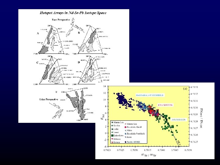
Figure 8. (a) after Pearce and Cann (1973), Earth Planet, Sci. Lett. , 19, 290 -300. (b) after Pearce (1982) in Thorpe (ed. ), Andesites: Orogenic andesites and related rocks. Wiley. Chichester. pp. 525 -548, Coish et al. (1986), Amer. J. Sci. , 286, 1 -28. (c) after Mullen (1983), Earth Planet. Sci. Lett. , 62, 53 -62.

Degree of melting, incompatible, compatible elements

REEs, spidergrams, HFSE, “anomalies” HFSE

Isotopes Same Z, different A (variable # of neutrons) 14 General notation for a nuclide: 6 C

Isotopes Same Z, different A (variable # of neutrons) 14 General notation for a nuclide: 6 C As n varies different isotopes of an element 12 C 13 C 14 C

HW 4 l l l Use the Cecil database to plot the incompatible trace element data relative to primitive mantle values for granitoids; do they exhibit any significant anomalies, are there any trends worthwhile interpreting? Determine the REE patterns (rel. to PM) and the magnitude of Eu anomalies; Use the Girardi et al 2012 paper as an example to make interpretations re the origin of magmas from the Rotberg area.

Stable Isotopes l l l Stable: last ~ forever Chemical fractionation is impossible Mass fractionation is the only type possible

Example: Oxygen Isotopes 16 O 17 O 18 O 99. 756% of natural oxygen 0. 039% “ 0. 205% “ Concentrations expressed by reference to a standard International standard for O isotopes = standard mean ocean water (SMOW)

18 O and 16 O are the commonly used isotopes and their ratio is expressed as d: d (18 O/16 O) = eq 9 -10 ( 18 O/ 16 O) sample - ( 18 O/ 16 O) SMOW 18 16 ( O/ O) SMOW result expressed in per mille (‰) What is d of SMOW? ? What is d for meteoric water? x 1000

What is d for meteoric water? Evaporation seawater vapor (clouds) Light isotope enriched in vapor > liquid F Pretty efficient, since D mass = 1/8 total mass F

What is d for meteoric water? Evaporation seawater vapor (clouds) Light isotope enriched in vapor > liquid F Pretty efficient, since D mass = 1/8 total mass F F d= ( 18 O/ 16 O) vapor - ( 18 O/ 16 O) SMOW 18 16 ( O/ O) SMOW x 1000 therefore ( 18 O/ 16 O) Vapor < ( 18 O/ 16 O) SMOW thus dclouds is (-)

Figure 9 -9. Relationship between d(18 O/16 O) and mean annual temperature for meteoric precipitation, after Dansgaard (1964). Tellus, 16, 436 -468.

Oxygen isotopes Can determine crustal recycling

Mantle-derived rocks = delta 18 O ~ 5 -6. 5 permil Crustal Rocks that have interacted with waters: Anything between -2 to +24 permil Oxygen has the mass advantage over other isotopes

Stable isotopes useful in assessing relative contribution of various reservoirs, each with a distinctive isotopic signature O and H isotopes - juvenile vs. meteoric vs. brine water F d 18 O for mantle rocks surface-reworked sediments: evaluate contamination of mantlederived magmas by crustal sediments F

Radioactive Isotopes l l Unstable isotopes decay to other nuclides The rate of decay is constant, and not affected by P, T, X… Parent nuclide = radioactive nuclide that decays Daughter nuclide(s) are the radiogenic atomic products

Isotopic variations between rocks, etc. due to: 1. Mass fractionation (as for stable isotopes) Only effective for light isotopes: H He C O S

Isotopic variations between rocks, etc. due to: 1. Mass fractionation (as for stable isotopes) 2. Daughters produced in varying proportions resulting from previous event of chemical fractionation 40 K 40 Ar by radioactive decay Basalt rhyolite by FX (a chemical fractionation process) Rhyolite has more K than basalt 40 K more 40 Ar over time in rhyolite than in basalt 40 Ar/39 Ar ratio will be different in each

Isotopic variations between rocks, etc. due to: 1. Mass fractionation (as for stable isotopes) 2. Daughters produced in varying proportions resulting from previous event of chemical fractionation 3. Time The longer 40 K 40 Ar decay takes place, the greater the difference between the basalt and rhyolite will be

Radioactive Decay The Law of Radioactive Decay d. N µN dt eq. 11 d. N or = l. N dt # parent atoms 1 ½ ¼ time

D = Nelt - N = N(elt -1) eq 14 age of a sample (t) if we know: D the amount of the daughter nuclide produced N the amount of the original parent nuclide remaining l the decay constant for the system in question

The appropriate decay equation is: eq 16 40 Ar = 40 Ar o æ le ö + çè ÷ø l 40 K(e-lt -1) Where le = 0. 581 x 10 -10 a-1 (proton capture) and l = 5. 543 x 10 -10 a-1 (whole process)

Sr-Rb System · 87 Rb 87 Sr + a beta particle (l = 1. 42 x 10 -11 a-1) · Rb behaves like K micas and alkali feldspar · Sr behaves like Ca plagioclase and apatite (but not clinopyroxene) · 88 Sr : 87 Sr : 86 Sr : 84 Sr ave. sample = 10 : 0. 7 : 1 : 0. 07 · 86 Sr is a stable isotope, and not created by breakdown of any other parent

Isochron Technique Requires 3 or more cogenetic samples with a range of Rb/Sr Could be: • 3 cogenetic rocks derived from a single source by partial melting, FX, etc. Figure 9 -3. Change in the concentration of Rb and Sr in the melt derived by progressive batch melting of a basaltic rock consisting of plagioclase, augite, and olivine. From Winter (2001) An Introduction to Igneous and Metamorphic Petrology. Prentice Hall.

Isochron Technique Requires 3 or more cogenetic samples with a range of Rb/Sr Could be: • 3 cogenetic rocks derived from a single source by partial melting, FX, etc. • 3 coexisting minerals with different K/Ca ratios in a single rock

Recast age equation by dividing through by stable 86 Sr = (87 Sr/86 Sr)o + (87 Rb/86 Sr)(elt -1) l = 1. 4 x 10 -11 a-1 87 Sr/86 Sr eq 9 -17 For values of lt less than 0. 1: elt-1 lt Thus eq. 9 -15 for t < 70 Ga (!!) reduces to: eq 9 -18 87 Sr/86 Sr y = (87 Sr/86 Sr)o + (87 Rb/86 Sr)lt = b + x = equation for a line in 87 Sr/86 Sr vs. 87 Rb/86 Sr plot m

Begin with 3 rocks plotting at a b c at time to 87 Sr 86 Sr ( ) 87 Sr 86 Sr o a b 87 Rb 86 Sr c to

After some time increment (t 0 t 1) each sample loses some 87 Rb and gains an equivalent amount of 87 Sr 86 Sr ( ) c 1 b 1 a 1 t 1 87 Sr 86 Sr o a b 87 Rb 86 Sr c to

At time t 2 each rock system has evolved new line Again still linear and steeper line t 2 87 Sr c 2 86 Sr b 2 a 2 ( ) c 1 b 1 a 1 t 1 87 Sr 86 Sr o a b c to 87 Rb 86 Sr

Isochron technique produces 2 valuable things: 1. The age of the rocks (from the slope = lt) 2. (87 Sr/86 Sr)o = the initial value of 87 Sr/86 Sr Figure 9 -9. Rb-Sr isochron for the Eagle Peak Pluton, central Sierra Nevada Batholith, California, USA. Filled circles are whole -rock analyses, open circles are hornblende separates. The regression equation for the data is also given. After Hill et al. (1988). Amer. J. Sci. , 288 -A, 213 -241.

Figure 9 -13. Estimated Rb and Sr isotopic evolution of the Earth’s upper mantle, assuming a large-scale melting event producing granitic-type continental rocks at 3. 0 Ga b. p After Wilson (1989). Igneous Petrogenesis. Unwin Hyman/Kluwer. .

The Sm-Nd System l Both Sm and Nd are LREE Incompatible elements fractionate melts F Nd has lower Z larger liquids > does Sm F

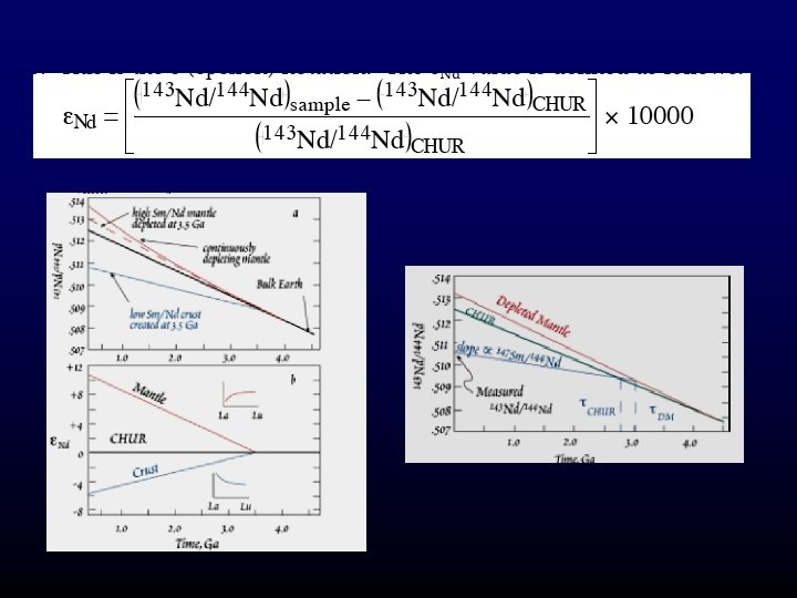
147 Sm 143 Nd by alpha decay l = 6. 54 x 10 -13 a-1 (half life 106 Ga) l Decay equation derived by reference to the non-radiogenic 144 Nd F 143 Nd/144 Nd = (143 Nd/144 Nd) o + (147 Sm/144 Nd)lt

Evolution curve is opposite to Rb - Sr Figure 9 -15. Estimated Nd isotopic evolution of the Earth’s upper mantle, assuming a large-scale melting or enrichment event at 3. 0 Ga b. p. After Wilson (1989). Igneous Petrogenesis. Unwin Hyman/Kluwer. .

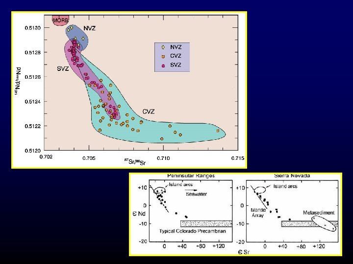
Systematic geographic distribution of isotopic ratios The 0. 706 line through the Sierra Nevada and north

Fractionation, assimilation, mixing

Simple Mixing Models Binary Ternary All analyses fall between two reservoirs as magmas mix All analyses fall within triangle determined by three reservoirs Figure 14 -5. Winter (2001) An Introduction to Igneous and Metamorphic Petrology. Prentice Hall.

HW 5 l l l Determine the initial Sr and Nd isotopes for the Cecil database; Plot the initial Sr vs. Nd isotopes, 87 Sr/86 Sr vs. 1/Sr and 143 Nd/144 Nd vs. 1/Nd; is there one or are there more sources of magmas? How many? Do the isotopes and isotope-elemental plots indicate any mixing curves? How many components? Plot at least one mixing line using Ig. Pet (or similar).

Other radiogenic systems and utilities l l l Pb-Pb (u and Th decay)- good for identifying sedimentary sources in magma (high U/Pb) He isotopes - can detect pristine, undegassed mantle in some plumes Ca isotopes - can trace old crustal components Hf isotopes - useless except perhaps when used in situ with U-Pb dating of zircons Re-Os - can effectively fingerprint crustal sources and date mantle events.

The U-Pb-Th System Very complex system. 3 radioactive isotopes of U: 234 U, 235 U, 238 U F 3 radiogenic isotopes of Pb: 206 Pb, 207 Pb, and 208 Pb 204 Pb is strictly non-radiogenic s Only F l l U, Th, and Pb are incompatible elements, & concentrate in early melts Isotopic composition of Pb in rocks = function of F F F 234 U 206 Pb 235 U 207 Pb 232 Th 208 Pb 238 U (l = 1. 5512 x 10 -10 a-1) (l = 9. 8485 x 10 -10 a-1) (l = 4. 9475 x 10 -11 a-1)

Common Pb

He isotopes