GEOS 28600 The science of landscapes Earth Planetary

GEOS 28600 The science of landscapes: Earth & Planetary Surface Processes http: //geosci. uchicago. edu/~kite/geos 28600_2019/ Lecture 6 Wednesday 30 Jan 2019 Wrap-up of The flow of ice Introduction to fluvial sediment transport

Logistics • Homework 2 is due now • No class next week due to NASA panel • Homework 3 will be issued no later than next Mon and will be due in class on Mon 11 Feb

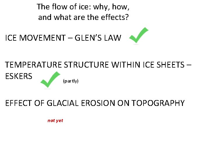
The flow of ice: why, how, and what are the effects? ICE MOVEMENT – GLEN’S LAW TEMPERATURE STRUCTURE WITHIN ICE SHEETS – ESKERS (partly) EFFECT OF GLACIAL EROSION ON TOPOGRAPHY not yet

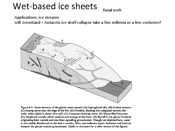
Wet-based ice sheets Basal melt Applications: ice streams will Greenland + Antarctic ice shelf collapse take a few millenia or a few centuries?

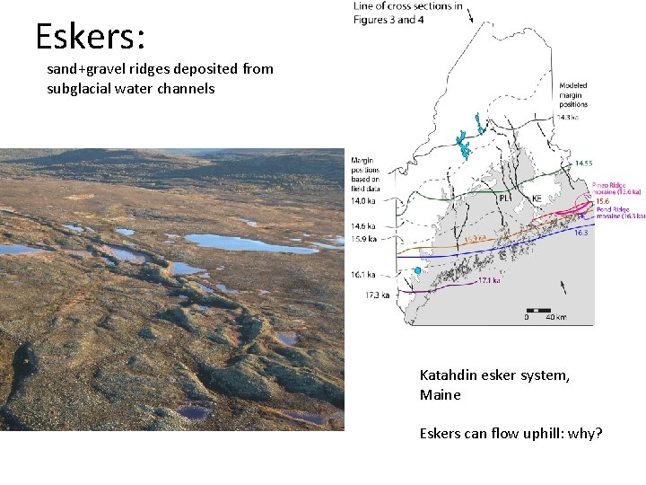
Eskers: sand+gravel ridges deposited from subglacial water channels Katahdin esker system, Maine Eskers can flow uphill: why?

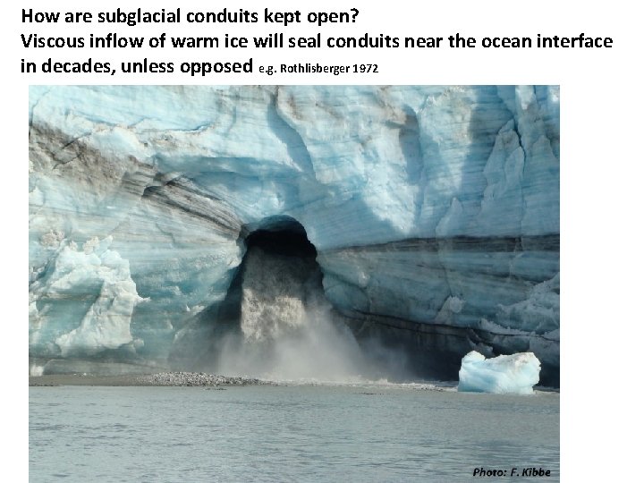
How are subglacial conduits kept open? Viscous inflow of warm ice will seal conduits near the ocean interface in decades, unless opposed e. g. Rothlisberger 1972

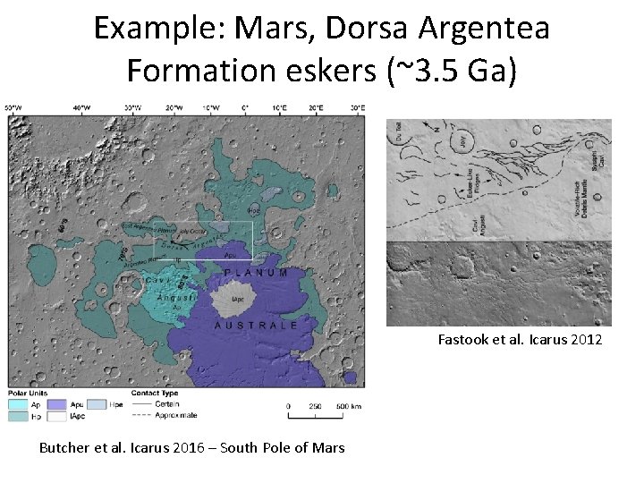
Example: Mars, Dorsa Argentea Formation eskers (~3. 5 Ga) Fastook et al. Icarus 2012 Butcher et al. Icarus 2016 – South Pole of Mars

The flow of ice ICE MOVEMENT – GLEN’S LAW TEMPERATURE STRUCTURE WITHIN ICE SHEETS – ESKERS (Mars examples) EFFECT OF GLACIAL EROSION ON TOPOGRAPHY (Earth examples)

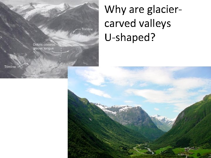
Why are glaciercarved valleys U-shaped?

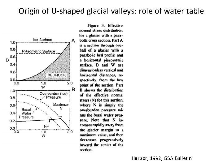
Origin of U-shaped glacial valleys: role of water table Harbor, 1992, GSA Bulletin

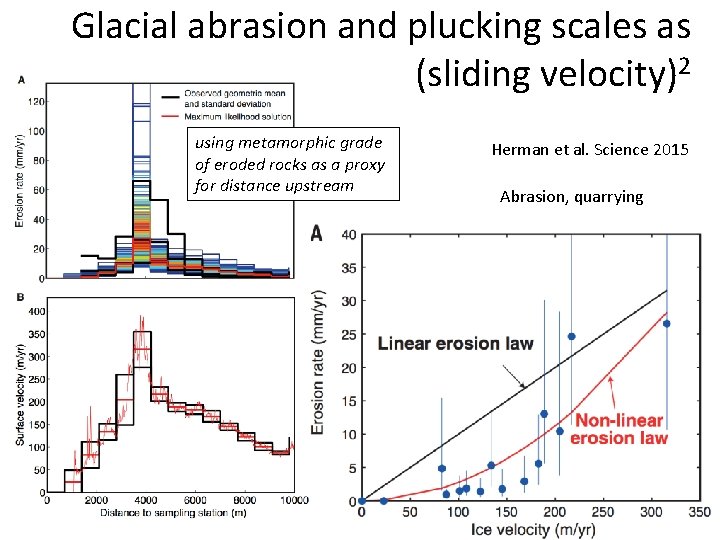
Glacial abrasion and plucking scales as (sliding velocity)2 using metamorphic grade of eroded rocks as a proxy for distance upstream Herman et al. Science 2015 Abrasion, quarrying

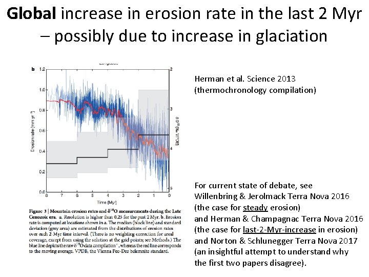
Global increase in erosion rate in the last 2 Myr – possibly due to increase in glaciation Herman et al. Science 2013 (thermochronology compilation) For current state of debate, see Willenbring & Jerolmack Terra Nova 2016 (the case for steady erosion) and Herman & Champagnac Terra Nova 2016 (the case for last-2 -Myr-increase in erosion) and Norton & Schlunegger Terra Nova 2017 (an insightful attempt to understand why the first two papers disagree).

Key points from “The Flow of Ice”: • Glen’s Law • Approximations to the full Stokes equation: locations where they are and are not acceptable • Nondimensional T-vs-depth as a function of accumulation rate for fixed basal heat flow • Glacial erosion parameterization

Fluvial sediment transport: introduction REVIEW OF LAB 2 and REQUIRED READING (SCHOOF & HEWITT 2013) TURBULENT VELOCITY PROFILES, INITIATION OF MOTION BEDLOAD, RIVER GEOMETRY

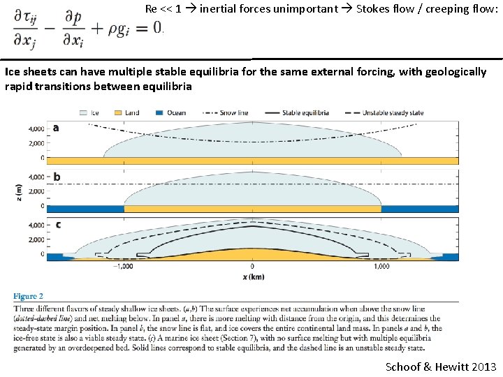
Re << 1 inertial forces unimportant Stokes flow / creeping flow: Ice sheets can have multiple stable equilibria for the same external forcing, with geologically rapid transitions between equilibria Schoof & Hewitt 2013

Key points from “Introduction to fluvial sediment transport”: • Critical Shields stress • Differences between gravel-bed vs. sand-bed rivers • Discharge-width scaling

Prospectus: fluvial processes • Today: overview, hydraulics. • Next lecture: initiation of motion, channel width adjustment. • Channel long-profile evolution. • Mountain belts. • Looking ahead: landscape evolution (including fluvial processes. ) This section of the course draws on courses by W. E. Dietrich (Berkeley), D. Mohrig (MIT U. T. Austin), and J. Southard (MIT).

Fluvial sediment transport: introduction REVIEW OF REQUIRED READING (SCHOOF & HEWITT 2013) TURBULENT VELOCITY PROFILES, INITIATION OF MOTION BEDLOAD, RIVER GEOMETRY

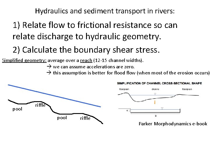
Hydraulics and sediment transport in rivers: 1) Relate flow to frictional resistance so can relate discharge to hydraulic geometry. 2) Calculate the boundary shear stress. Simplified geometry: average over a reach (12 -15 channel widths). we can assume accelerations are zero. this assumption is better for flood flow (when most of the erosion occurs). pool riffle Parker Morphodynamics e-book

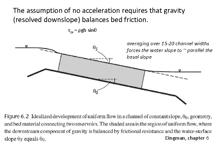
The assumption of no acceleration requires that gravity (resolved downslope) balances bed friction. τzx = ρgh sinθ averaging over 15 -20 channel widths forces the water slope to ~ parallel the basal slope Dingman, chapter 6

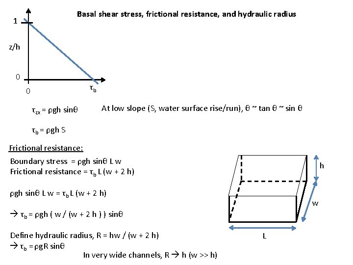
Basal shear stress, frictional resistance, and hydraulic radius 1 z/h 0 τb 0 τzx = ρgh sinθ At low slope (S, water surface rise/run), θ ~ tan θ ~ sin θ τb = ρgh S Frictional resistance: Boundary stress = ρgh sinθ L w Frictional resistance = τb L (w + 2 h) h ρgh sinθ L w = τb L (w + 2 h) w τb = ρgh ( w / (w + 2 h ) ) sinθ Define hydraulic radius, R = hw / (w + 2 h) τb = ρg. R sinθ In very wide channels, R h (w >> h) L

Law of the wall, recap: Glaciers ( Re << 1): Rivers ( Re >> 10, and fully turbulent): τzx = ρ KT (du/dz) τzx = μ(T, σ) (du/dz) eddy viscosity, “diffuses” velocity Properties of turbulence: Irregularity From empirical & theoretical studies: Diffusivity Vorticity KT = (k z )2 (du/dz) (where k = 0. 39 -0. 4 = von Karman’s constant) Dissipation τB = ρ(k z)2 (du/dz)2 (τB /ρ )1/2 = k z (du / dz) = u* = “shear velocity” Memorize this. (ρ g h S /ρ )1/2 = u* = ( g h S )1/2 Now u* = k z (du / dz) Separate variables: du = (u* / k z ) dz Integrate: u = (u*/k) (ln z + c). For convenience, set c = -ln(z 0) “law of the wall” Then, u = (u*/k) ln (z/z 0) when z = z 0, u = 0 m/s. (explained on next slide)

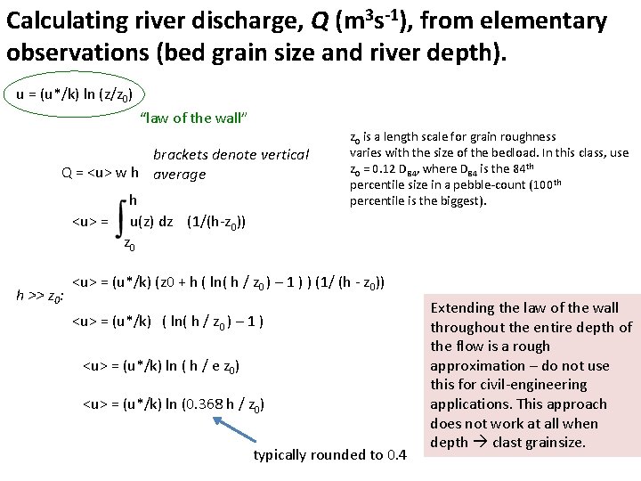
Calculating river discharge, Q (m 3 s-1), from elementary observations (bed grain size and river depth). u = (u*/k) ln (z/z 0) “law of the wall” brackets denote vertical Q = <u> w h average h <u> = u(z) dz (1/(h-z 0)) z 0 h >> z 0: z 0 is a length scale for grain roughness varies with the size of the bedload. In this class, use z 0 = 0. 12 D 84, where D 84 is the 84 th percentile size in a pebble-count (100 th percentile is the biggest). <u> = (u*/k) (z 0 + h ( ln( h / z 0 ) – 1 ) ) (1/ (h - z 0)) <u> = (u*/k) ( ln( h / z 0 ) – 1 ) <u> = (u*/k) ln ( h / e z 0) <u> = (u*/k) ln (0. 368 h / z 0) typically rounded to 0. 4 Extending the law of the wall throughout the entire depth of the flow is a rough approximation – do not use this for civil-engineering applications. This approach does not work at all when depth clast grainsize.

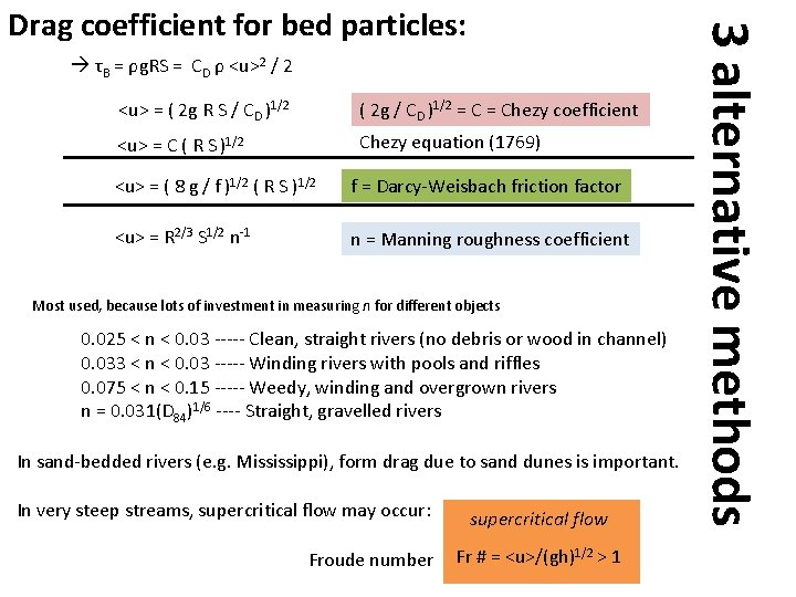
τB = ρg. RS = CD ρ <u>2 / 2 <u> = ( 2 g R S / CD )1/2 ( 2 g / CD )1/2 = Chezy coefficient <u> = C ( R S )1/2 Chezy equation (1769) <u> = ( 8 g / f )1/2 ( R S )1/2 f = Darcy-Weisbach friction factor <u> = R 2/3 S 1/2 n-1 n = Manning roughness coefficient Most used, because lots of investment in measuring n for different objects 0. 025 < n < 0. 03 ----- Clean, straight rivers (no debris or wood in channel) 0. 033 < n < 0. 03 ----- Winding rivers with pools and riffles 0. 075 < n < 0. 15 ----- Weedy, winding and overgrown rivers n = 0. 031(D 84)1/6 ---- Straight, gravelled rivers In sand-bedded rivers (e. g. Mississippi), form drag due to sand dunes is important. In very steep streams, supercritical flow may occur: Froude number supercritical flow Fr # = <u>/(gh)1/2 > 1 3 alternative methods Drag coefficient for bed particles:

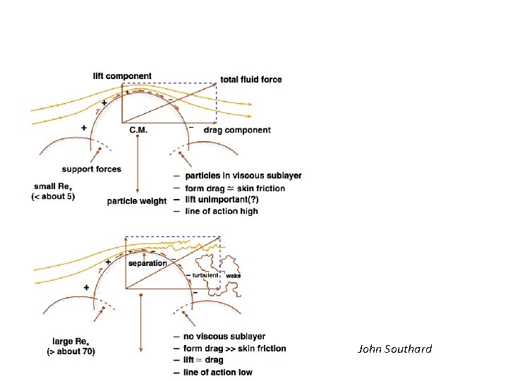
Getting from water flow to sediment flux

John Southard

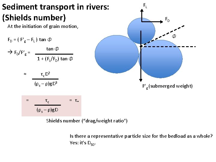
Sediment transport in rivers: (Shields number) FL FD At the initiation of grain motion, Φ FD = ( F’g – FL ) tan Φ FD/F’g = ≈ tan Φ 1 + (FL/FD) tan Φ τ c D 2 (ρs – ρ)g. D 3 = τc F’g (submerged weight) = τ* (ρs – ρ)g. D Shields number (“drag/weight ratio”) Is there a representative particle size for the bedload as a whole? Yes: it’s D 50.

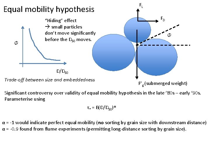
Equal mobility hypothesis Φ “Hiding” effect small particles don’t move significantly before the D 50 moves. FL FD Φ D/D 50 Trade-off between size and embeddedness F’g (submerged weight) Significant controversy over validity of equal mobility hypothesis in the late ’ 80 s – early ’ 90 s. Parameterise using τ* = B(D/D 50)α α = -1 would indicate perfect equal mobility (no sorting by grain size with downstream distance) α = -0. 9 found from flume experiments (permitting long-distance sorting by grain size).

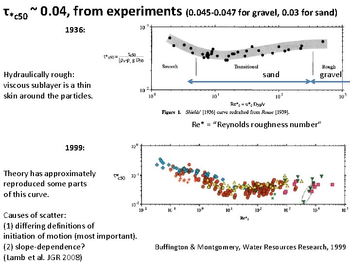
τ*c 50 ~ 0. 04, from experiments (0. 045 -0. 047 for gravel, 0. 03 for sand) 1936: Hydraulically rough: viscous sublayer is a thin skin around the particles. sand gravel Re* = “Reynolds roughness number” 1999: Theory has approximately reproduced some parts of this curve. Causes of scatter: (1) differing definitions of initiation of motion (most important). (2) slope-dependence? (Lamb et al. JGR 2008) Buffington & Montgomery, Water Resources Research, 1999

Fluvial sediment transport: introduction REVIEW OF REQUIRED READING (SCHOOF & HEWITT 2013) TURBULENT VELOCITY PROFILES, INITIATION OF MOTION BEDLOAD, RIVER GEOMETRY

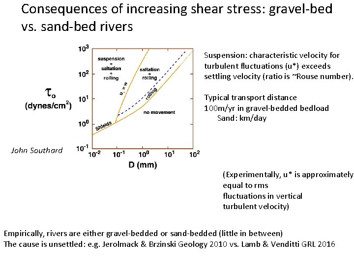
Consequences of increasing shear stress: gravel-bed vs. sand-bed rivers Suspension: characteristic velocity for turbulent fluctuations (u*) exceeds settling velocity (ratio is ~Rouse number). Typical transport distance 100 m/yr in gravel-bedded bedload Sand: km/day John Southard (Experimentally, u* is approximately equal to rms fluctuations in vertical turbulent velocity) Empirically, rivers are either gravel-bedded or sand-bedded (little in between) The cause is unsettled: e. g. Jerolmack & Brzinski Geology 2010 vs. Lamb & Venditti GRL 2016

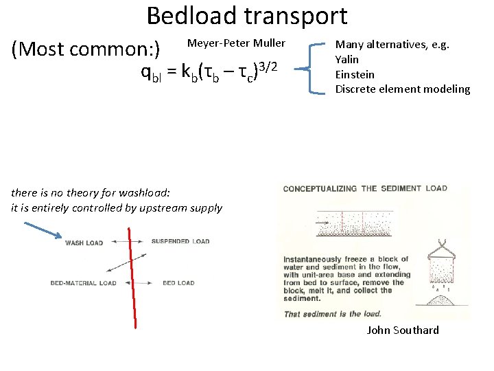
Bedload transport (Most common: ) Meyer-Peter Muller qbl = kb(τb – τc)3/2 Many alternatives, e. g. Yalin Einstein Discrete element modeling there is no theory for washload: it is entirely controlled by upstream supply John Southard

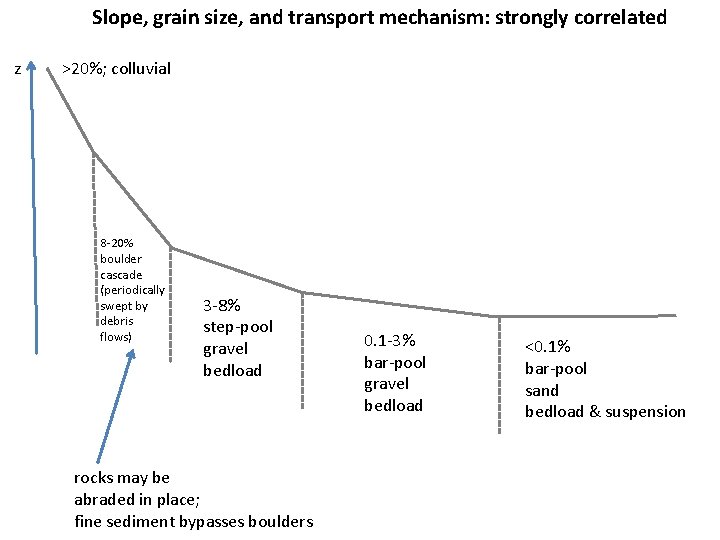
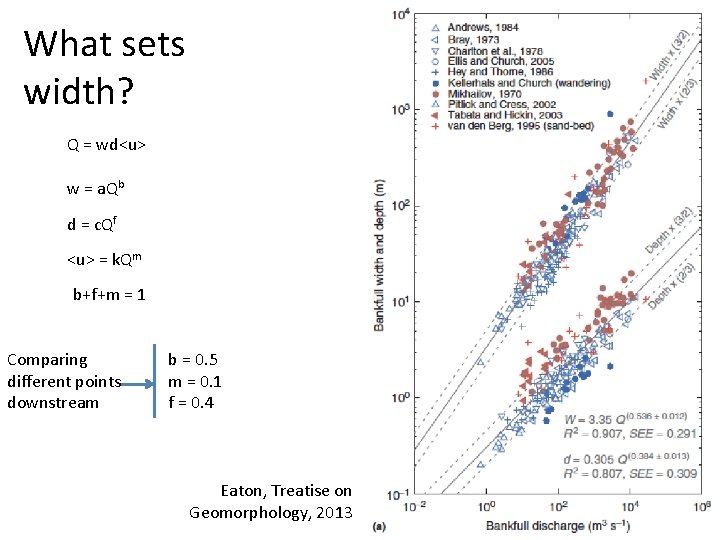
River channel morphology and dynamics • “Rivers are the authors of their own geometry” (L. Leopold) – And of their own bed grain-size distribution. • • Rivers have well-defined banks. – Bankfull discharge 5 -7 days per year; floodplains inundated every 1 -2 years. – Regular geometry also applicable to canyon rivers. – Width scales as Q 0. 5 River beds are (usually) not flat. – Plane beds are uncommon. Bars and pools, spacing = 5. 4 x width. • Rivers meander. – Wavelength ~ 11 x channel width. • River profiles are concave-up. – Grainsize also decreases downstream.

Slope, grain size, and transport mechanism: strongly correlated z >20%; colluvial 8 -20% boulder cascade (periodically swept by debris flows) 3 -8% step-pool gravel bedload rocks may be abraded in place; fine sediment bypasses boulders 0. 1 -3% bar-pool gravel bedload <0. 1% bar-pool sand bedload & suspension

What sets width? Q = wd<u> w = a. Qb d = c. Qf <u> = k. Qm b+f+m = 1 Comparing different points downstream b = 0. 5 m = 0. 1 f = 0. 4 Eaton, Treatise on Geomorphology, 2013

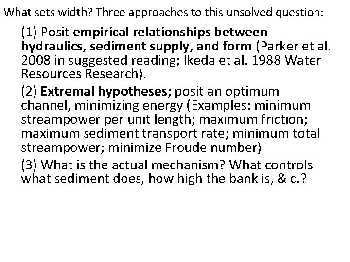
What sets width? Three approaches to this unsolved question: (1) Posit empirical relationships between hydraulics, sediment supply, and form (Parker et al. 2008 in suggested reading; Ikeda et al. 1988 Water Resources Research). (2) Extremal hypotheses; posit an optimum channel, minimizing energy (Examples: minimum streampower per unit length; maximum friction; maximum sediment transport rate; minimum total streampower; minimize Froude number) (3) What is the actual mechanism? What controls what sediment does, how high the bank is, & c. ?

Key points from “Introduction to fluvial sediment transport” • Law of the wall – how to calculate river discharge from elementary measurements (bed grain size and river depth). • Critical Shields stress • Differences between gravel-bed vs. sand-bed rivers • Discharge-width scaling

Bonus slides

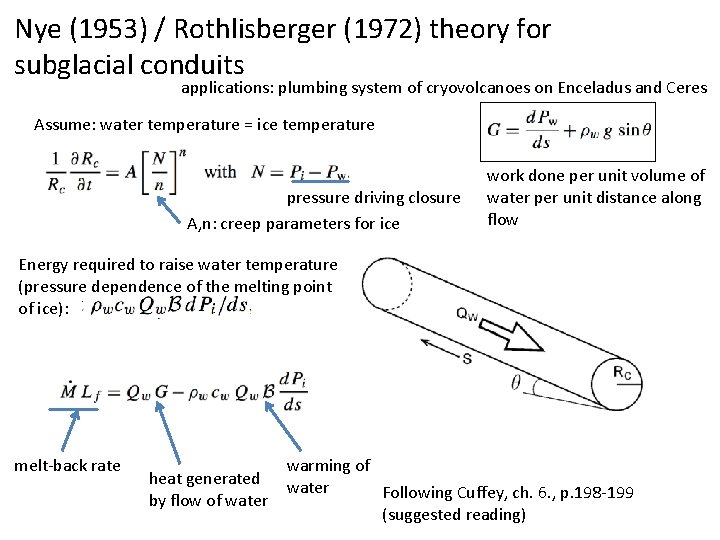
Nye (1953) / Rothlisberger (1972) theory for subglacial conduits applications: plumbing system of cryovolcanoes on Enceladus and Ceres Assume: water temperature = ice temperature pressure driving closure A, n: creep parameters for ice work done per unit volume of water per unit distance along flow Energy required to raise water temperature (pressure dependence of the melting point of ice): melt-back rate heat generated by flow of water warming of water Following Cuffey, ch. 6. , p. 198 -199 (suggested reading)

Pressure reduction in big Rothlisberger channels causes them to parasitize flow from smaller channels